Regression analysis is a statistical technique commonly used in the social and physical sciences to model relationships between variables. To make unbiased, consistent, and efficient inferences about real-world relationships a researcher using regression analysis relies on a set of assumptions about the process generating the data used in the analysis and the errors produced by the model. Several of these assumptions are frequently violated when the real-world process generating the data used in the regression analysis is spatially structured, which creates dependence among the observations and spatial structure in the model errors. To avoid the confounding effects of spatial dependence, spatial autoregression models include spatial structures that specify the relationships between observations and their neighbors. These structures are most commonly specified using a weights matrix that can take many forms and be applied to different components of the spatial autoregressive model. Properly specified, including these structures in the regression analysis can account for the effects of spatial dependence on the estimates of the model and allow researchers to make reliable inferences. While spatial autoregressive models are commonly used in spatial econometric applications, they have wide applicability for modeling spatially dependent data.
Author and Citation Info:
Hoffman, T. D. and Kedron, P. (2023). Spatial Autoregressive Models. The Geographic Information Science & Technology Body of Knowledge (2nd Quarter 2023 Edition). John P. Wilson (Ed.). DOI: https://doi.org/10.22224/gistbok/2023.2.1
This Topic is also available in the following editions: DiBiase, D., DeMers, M., Johnson, A., Kemp, K., Luck, A. T., Plewe, B., and Wentz, E. (2006). Bayesian methods. The Geographic Information Science & Technology Body of Knowledge. Washington, DC: Association of American Geographers. (2nd Quarter 2016, first digital)
Spatial weights matrix: A matrix W of entries wij that quantify the spatial relationship between locations i and j. These can take the form of binary contiguity weights (wij = 1 if iand j are related and 0 otherwise), kernel weights (wij is a non-increasing function of the distance between iand j), or empirical weights (wij is defined by another dataset), among others.
Regression: A statistical technique that relates a set of predictor or independent variables (denoted by X), to a response or dependent variable (denoted by y) via an algebraic equation specified by a researcher.
Spatial dependence: A spatial variable is said to be spatially dependent when values of the variable at one location are affected by values of that variable at nearby locations.
Spatial autoregressive structure: A mathematical representation of the relationship between values of a variable at different locations meant to reflect real-world spatial dependencies.
Direct effect: The nonspatial relationship between a predictor variable and the response variable, i.e., the extent to which a predictor variable affects the response variable.
Indirect effect: The spatial relationship between a variable and the response variable, i.e., the extent to which the spatial distribution of a variable affects the response variable, excluding the direct effect.
When studying the world, researchers are often interested in predicting unobserved instances of a phenomenon and/or identifying the relationships that may be creating that phenomenon. In many research settings, regression analysis acts as a stepping stone for inferences about how one variable affects another, and whether that estimated relationship merits a causal interpretation or can be reliably used to predict phenomena yet to be observed. To make unbiased, consistent, and efficient inferences about real-world relationships, a researcher using regression analysis relies on a set of assumptions. However, the key assumption that observations used in a regression analysis are independent and identically distributed is frequently violated in many research settings because the real-world process generating those observations is spatially structured. More often real-world processes create observations that are spatially dependent. A situation in which values observed at one location or region are affected by values of neighboring observations at nearby locations (Anselin, 1989).
Spatial autoregressive models (SAMs) are a parsimonious way of accounting for the spatial dependence that often exists in geographic research. In a SAM a researcher introduces a spatial relationship into their regression analysis that defines how they believe values in different locations affect one another. Ideally, the researcher will select a mathematical formulation of the relationship that closely matches the true spatially structured process responsible for the observed data. However, a wide range of processes can create spatially dependent observations, which has motivated the development of a variety of forms of SAM (Section 3).
Perhaps the most intuitive motivation for the use of a SAM is the presence of spillover effects across locations. For example, prices in the housing market are typically estimated using hedonic price models that attribute the price of a home to its different characteristics. While the number of bedrooms in a home may determine its price, so too do the price of homes with similar characteristics sold in nearby areas. Using a SAM, a researcher can represent the effect surrounding homes prices have on the price of a home by including a spatially lagged price variable as a predictor variable in their regression analysis. Similarly, if a researcher believes that the condition of the property of surrounding homes may impact the price of a home, they can include those features as spatially lagged predictors in their regression analysis. In both cases the researcher is imposing a spatially autoregressive structure onto their regression analysis. However, in the first instance they are including a surrounding response variable (price) while in the second they are including a surrounding predictor variable (property condition).
Another key motivation for the use of SAM is to avoid the potential for omitted variable bias. Omitted variables bias occurs when a researcher leaves one or more relevant variable out of a statistical model. Returning to the housing market example, it is often the case that variable such as neighborhood reputation affects home prices but are difficult to measure and include in an analysis. If this variable is not included in the analysis and are spatially independent, a normal regression analysis remains unbiased. However, if the omitted variable is spatially dependent, and the reputation of one neighborhood does impact the reputation of those surrounding it, failing to include that dependence in the statistical model inflates the variance of the regression estimates reducing the efficiency of the model. If the omitted variable is also correlated with the predictor variables included in the regression analysis, which is likely to be the case for many real-world processes, the model estimates are also biased.
If a researcher used a nonspatial regression analysis to examine each of the problems above, their analysis would produce improper estimates of the relationships they seek to understand (Cressie, 1991). SAMs are an established statistical framework for estimated variable relationships when observations are spatially dependent (LeSage and Pace, 2009).
Regression analysis is a flexible statistical technique that researchers can use to estimates relationships between a response variable and one or more predictor variables. Regression models are expressed as algebraic equations
(Equation 1)
that consist of how a linear combination of predictor variables X, multiplied by parameters βthat represent the strength of each variable’s effect on a response variable y, and an error term ε (Hastie et al., 2008). The most commonly used form of regression, linear regression, models continuous response variables, but this form can be adapted to model other types of response variables (e.g., logistic regression for modeling binary responses).
Conventional regression assumes that the n observations included in the analysis are independent and identically distributed. However, spatial data routinely violates this assumption as nearby observations are likely to affect each other’s values (Anselin, 1989). One way to include these dependencies in the regression analysis would be to specify the unique covariance structure that exists between each observation and every other observation. However, this approach would require the specification and estimation of (n2-n) relationships among the n locations, ruling out dependence of an observation on itself (Bailey and Gatrell, 1995). This approach is impractical in nearly all situations. Building on Whittle (1954), Ord (1975) proposed imposing a simplified structure on these many spatially dependent relationships as a tractable solution to this over-parameterization problem. The structure introduced into the model is known as a spatial autoregressive process.
2.2 The Spatial Autoregressive Structure
When a spatial autoregressive structure is imposed upon a variable, the spatial dependence relationships that exist between observations are simplified and introduced into the model using an n x n spatial weights matrix W. The spatial weights matrix can take many forms (e.g., contiguity, nearest neighbors, distance), but in each instance the matrix constrains within the model how observations are. This constraint simplifies the estimation of covariance among locations. Applied to the spatially dependent observations of the response variable y, the spatial autoregressive process can be represented as
(Equation 2)
where ρ represents the level of global spatial autocorrelation present in y and εis a n×1 vector of nonspatial independent and identically distributed random errors. The matrix-vector product Wy is a spatially weighted average of the values of Y that is limited by the form of the spatial weights matrix.
Through matrix algebra, Equation 2 can be rearranged to yield , a more compact expression for the autoregressive nature of the model. The factor can be thought of as a spatial autocorrelation operator with global spatial autocorrelation level ρ. All SAMs use some form of this operator to capture the spatial dependence among observations.
The spatial autoregressive structure, and its characteristic factor, can be applied to the response (y), predictors (X), and error (ε) components of the traditional regression equation creating a flexible framework for analysis. The matrix multiplication of the weights matrix W with a covariate is called a spatial lag, and represents a linear combination of the values of that component and neighboring observations (as defined by the weights matrix). This multiplication expresses the spatial dependence among locations by replacing the value of a variable at a location with a spatially weighted average of its neighbors’ values. For example, if there are n locations in the study area, a spatial lag of the predictor variables is the left-multiplication of the n×n spatial weights matrix on the predictors X, which generates the n×k spatial lag WX . For the response variable y the same procedure generates a n×1 spatial lag Wy. As above, these spatially lagged terms are accompanied by parameters, ρ for lags of the response variable and γ for lags of the predictor variables, that capture the strength of the spatial autocorrelation among those observations of that variable. Often, the spatial weights matrix used during model estimation is standardized, or transformed in a way to preserve certain properties. Row standardization - ensuring the rows of W sum to 1 - is the most common of these but is not always the most preferable (see Elhorst, 2014 for details).
Applied to the error component of a regression analysis, a spatial autoregressive structure segments the error, ε, of a nonspatial regression y=Xβ+ε into two parts: a spatially autocorrelated term and a nonspatial term. To do this, the nonspatial regression is rewritten as y=Xβ+u and the error is decomposed as u=λWu+ε where λ is a parameter to be calibrated and ε is a n×1 vector of independent and identically distributed normal nonspatial errors. Estimates of the parameter λ express the average strength of spatial autocorrelation among the errors conditional on W.
The inclusion and exclusion of a spatial lagged response, spatial lagged predictors, and the spatial error decomposition define a taxonomy of SAM specifications (Fig. 1). Each combination of the lagged components defines a different SAM and different form of spatial dependence. Branching out from the classic ordinary least squares (OLS) regression (Fig. 1a), the most basic SAMs are the spatial lag of X model (SLX – Fig. 1b), and the spatial error model (SEM – Fig. 1c), and the lag model (SAR – Fig. 1d). Each of these models includes only one of the lag components presented above. The SLX model introduces the spatial lag WX of the predictors and the vector of parameters γ. The SAR model includes the spatial lag Wy of the response variable and the scalar parameter ρ. The SEM partitions the error terms and adds the scalar parameter λ.
Figure 1. Taxonomy of spatial autoregressive models. Arrows illustrate how the progressive addition of spatially lagged components to ordinary least square regression analysis increase specification complexity. Adapted from Elhorst (2014). Source: authors.
Crucially, the use of these models should be matched to a researcher's conceptualization of the spatially structured real-world process they believe to be responsible for the observed data. For example, the housing price examples presented in the motivation section can be matched to each model. If a researcher is modeling home prices and believes the price of surrounding homes affects home prices, they would select the SAR model. The SLX model would match the case where the condition of surrounding properties impacts price, and the SEM model for the case where unmeasured neighborhood reputation impacts price.
In many cases a researcher may believe that multiple spatially dependent factors shape the data generating process. To accommodate these situations, the next layer of SAMs includes multiple lagged components. The Kelejian-Prucha model (SAC – Fig. 1e) combines a spatial lag of y and the spatial error component. The Spatial Durbin model (SDM – Fig. 1f) includes spatial lags of X and y , while the spatial Durbin error model (SDEM – Fig. 1g) includes a spatial lag of X and a spatial error component. These models express increasingly complex forms of spatial dependence among the data and nest the more parsimonious SAR, SLX, and SEM models within them. Inclusion of all three spatially lagged components produces the generalized nesting spatial model (GNS). However, the GNS specification, which is similar to the Manski neighborhood effects model (Manski, 1993), is not often commonly used in empirical work for reasons presented below.
There is debate as to whether several forms of SAM can be meaningfully applied to many real-world processes and how to properly interpret the relationships estimated by these models (see Pinske and Slade, 2010; Gibbons and Overman, 2012; LeSage, 2014). The debate centers on the difficult task of properly specifying the spatially dependent structures of the data generating process and how different SAMs incorporate local versus global spillover effects into the model. On the first point, in practice researchers often do not have a detailed understanding of the many interacting processes creating an observed phenomenon. If a researcher uses a SAM that models the processes too simplistically, the effects of spatial dependence may not be accounted for. Alternatively, if a researcher uses an overly complex SAM they may overfit their model. The parameter estimates of an overfitted model are not meaningful because they incorporate some of the variation in the residuals as if that variation reflected model structure (for further discussion see LeSage and Pace, 2014; Ver Hoef et al., 2018; Kedron et al., 2022).
SAM specification is further complicated by the two types of spatial dependencies or spillovers that are introduced by including different spatially lagged components in the model. Including a spatial lag of the predictor Wy into a SAM introduces a global spillover effect such that a change in a predictor X in any location will affect the response y in all other locations. This global effect exists even when the spatial weights matrix constrains spatial dependence to a subset of nearby regions. This is the case because each the response variable observed at each location affects its surrounding neighbors, which in turn affect their surrounding neighbors, and so on. These dependencies create a progressively diminishing but rippling indirect effect of the change in the predictor across the entire study area. A locally constrained version of this process occurs when WX is included in a SAM. In this case a change in the value of the predictor in one location affects that location's response variable, and those in the surrounding areas. As long as the SAM does not include a spatially lagged response variable, the ripple effects end in those neighboring regions.
Crucially, in the case of both local and global spillovers the estimated parameter values of γ and ρ associated with the spatially lagged predictor or response variables capture of both direct and indirect effects. As such these estimates cannot be interpreted as β estimates in OLS regression that indicate the change in response variable associated with a unit change in the predictor variable. Direct effects are the product of the relationship between a predictor and response variable and are interpretable like conventional OLS parameter estimates. In contrast, indirect effects are the global or local spatial spillover effects that extend beyond the direct effect and across locations. Golgher and Voss (2016) provide the derivation of each type of effect for different SAMs and discuss further how to interpret indirect effects.
Considering both the challenge of model specification and the need to differentiate direct and indirect effects, LeSage (2014) argues that the SDM and SDEM are the SAMs that best lend themselves to meaningful interpretation. As such, LeSage recommends a specification procedure rooted in a researcher's belief about whether global or local spillovers are likely driving the process under study. If a researcher believes spatial dependencies are local, they can begin with the SDEM model which will allow them to work back up the SAM taxonomy and make comparisons to more parsimonious SEM, SLX, and OLS models. If a researcher believes the spatial dependencies of the process under study are global, they can begin with the SDM model and make comparisons to SLX, SAR, and OLS models. Alternatively, the GNS is not commonly used as the starting point for applied work because it is only weakly identifiable, generating higher uncertainty in parameter estimates (Gibbons and Overman, 2012), and when identifiable may often be overparameterized (Burridge et al. 2016). Plainly, the inclusion of all possible spatial effects makes it difficult to interpret and reliably estimate any single spatial effect. As such, the GNS is not a viable alternative compared to the SDM or SDEM for the starting point of a data analysis.
Spatial dependence complicates the estimation of SAM parameters as compared to a standard OLS model (Fischer and Wang, 2011). Initial computationally expensive SAM estimation techniques involved direct maximum likelihood estimation (Ord, 1975). Maximum likelihood estimation utilizes a function that describes the likelihood of a set of parameters given the data. The form of the likelihood function is determined by the specification of the SAM being fit. The fitting procedure optimizes the likelihood function using numerical optimization techniques. A SAM's estimated parameters are those that generate the highest likelihood of observing the data under a given model specification.
However, the likelihood function often takes a form that is not conducive to straightforward optimization. To circumvent these difficulties, some estimation techniques exploit aspects of the model structure for computational complexity, accuracy, and speed. These often use sparse matrix operations or quasi-likelihood functions that approximate the true likelihood function (e.g., Pace and Berry, 1997). Computational innovations in the estimation procedure have contributed to the widespread use and scalability of spatial autoregressive models in geographical and econometric research. Due to these techniques and modern computer architectures, SAMs can accept tens of thousands to hundreds of thousands of observations with little effect on the time needed to fit the models.
While modern estimation routines are sophisticated maximum likelihood methods (Kelejian and Prucha, 2007; Arraiz et al., 2010; Drukker et al., 2010), other estimation techniques have seen development in spatial autoregressive models. Among these techniques are generalized method of moments estimators (Kelejian and Prucha, 1998; Kelejian and Prucha, 1999; Lee, 2003; Lee, 2004), Bayesian approaches (LeSage and Pace, 2009), instrumental variables (Anselin, 1980), and spatial filtering methods (Griffith, 2003). More broadly, the recommended estimation technique for SAM is to begin with the generalized method of moments before proceeding to alternatives such as maximum likelihood estimation (Anselin and Rey, 2014).
There are a variety of software programs capable of implementing SAMs. Open source code for SAMs can be found in the spreg package of the Python Spatial Analysis Library (PySAL; https://pysal.org/spreg/), the spatialreg package of the R-Spatial ecosystem (https://cran.r-project.org/web/packages/spatialreg/index.html), or the Spatial Econometrics Toolbox in MATLAB (https://www.spatial-econometrics.com/). Beyond the source code, GeoDa is a graphical user interface that enables a variety of spatial data analyses including spatial regression (https://geodacenter.github.io/; Anselin and Rey, 2014). These packages and interfaces offer varying levels of abstraction to users and not all provide the separate estimates of direct and indirect effects needed for model interpretation.
The hallmark feature of SAMs is that they model spatial structure simultaneously—random variables appear on both sides of the model equations. In the spatially-lagged y model (for example), the same random variable yi simultaneously appears on the left side of the ith regression equation and on the right side of the equations of neighbors of i. This paradigm (termed simultaneous autoregressive, or SAR, modeling) is the source of many of the issues of interpretation discussed in Section 4: the set of regression equations must be solved differently from a nonspatial regression to account for the simultaneously occurring variables (Smith, 2014). However, the matrix equations produced by SAR models are simple to conceptualize in the context of nonspatial regression, which has facilitated their widespread use.
Alternatively, analysts may model spatial structure conditionally, whereby the random variable y at location iis conditionally dependent on neighboring values of y (Ver Hoef et al., 2018). That is, a model is specified for the probability distribution of yi given the values of its neighbors. While this generates a more complex set of regression equations, the conditional formulation enables Bayesian inference and allows for the specification of hierarchical spatial models (Banerjee et al., 2014; Smith, 2014). The SAR and CAR models are equivalent under certain assumptions, but generally represent different ways of thinking about spatial structure and thus produce different conclusions for modelers (Cressie, 1991).
Spatial autoregressive modeling is an established and flexible statistical framework that researchers can use to estimate variable relationships when observations are spatially dependent. A number of alternative SAM specifications are available to researchers, although selection among these alternatives and proper specification can be challenging. A researcher must choose what components of the regression model need to be spatially lagged and create a spatial weights matrix that identifies how spatial dependencies in those components are structured. Both choices can dramatically impact the estimates of a SAM (LeSage 2009, Harris et al. 2011). Ultimately, the use and proper specification of SAMs is the responsibility of the researcher who must choose the model form that best represents their conceptualization of the relationships and spatial dependencies relevant to the phenomena they are studying. If properly specified, SAMs can provide reliable estimates of the relationships between variables in the presence of a spatially structured data generating process.
References:
Anselin, L. (1980). Estimation methods for spatial autoregressive structures. Regional Science Dissertation and Monograph Series, Cornell University, Ithaca, NY.
Anselin, L. (1988). Spatial Econometrics: Models and Methods. Norwell, MA: Kluwer Academic Publishers.
Anselin, L. (1989). What is Special About Spatial Data? Alternative Perspectives on Spatial Data Analysis. UC Santa Barbara NCGIA Technical Reports, 89-4.
Anselin L., and Rey S.J. (2014) Modern spatial econometrics in practice: A guide to GeoDa, GeoDaSpace and PySAL. GeoDa Press LLC.
Arraiz I, Drukker D.M., Kelejian H.H., Prucha I.R. (2010). A Spatial Getis-Ord-type Model with Heteroscedastic Innovations: Small and Large Sample Results. Journal of Regional Science, 50, 592–614.
Bailey, T.C., and Gatrell, A.C. (1995). Interactive spatial data analysis. Longman Scientific & Technical, New York.
Banerjee, S., Carlin, B.P., and Gelfand, A.E. (2014). Hierarchical Modeling and Analysis for Spatial Data, 2ndedition. Chapman and Hall/CRC Press Monographs on Statistics and Applied Probability, Boca Raton, FL.
Bivand, R. (2017). Revisiting the Boston data set – Changing the units of observation affects estimated willingness to pay for clean air. Region, 4 (1), 109-127.
Burridge, P., Elhorst, J.P., and Zigova, K. (2016). Group Interactions in Research and the Use of General Nesting Spatial Models. In B.H. Batagi, J.P. LeSage, and R.K. Pace (eds.), Spatial Econometrics: Quantitative and Limited Dependent Variables (Vol. 37, 223-258). Emerald Group Publishing Limited.
Cressie, N. (1991). Statistics for Spatial Data. Wiley Series in Probability and Mathematical Statistics.
Drukker, D.M., Egger, P., and Prucha, I.R. (2010). On Two-step Estimation of a Spatial Autoregressive Model with Autoregressive Disturbances and Endogenous Regressors. Available here.
Elhorst, J. P. (2014). Linear Spatial Dependence Models for Cross-Section Data. In Spatial Econometrics, by J. Paul Elhorst, 5–36. SpringerBriefs in Regional Science. Berlin, Heidelberg: Springer Berlin Heidelberg. https://doi.org/10.1007/978-3-642-40340-8_2.
Fischer, M.M., and Wang, J. (2011). Spatial Data Analysis: Models, Methods, and Techniques. Springer.
Golgher, A. B., and Voss, P.R. (2016). How to Interpret the Coefficients of Spatial Models: Spillovers, Direct and Indirect Effects. Spatial Demography 4 (3), 175–205. https://doi.org/10.1007/s40980-015-0016-y.
Griffith, D.A. (2003) Spatial autocorrelation and spatial filtering: Gaining understanding through theory and scientific visualization. Springer Verlag, Berlin.
Halleck Vega, S. and Elhorst, P. (2013). On spatial econometric models, spillover effects, and W, 53rd Congress of the European Regional Science Association: "Regional Integration: Europe, the Mediterranean and the World Economy", 27-31 August 2013, Palermo, Italy, European Regional Science Association (ERSA), Louvain-la-Neuve.
Hastie, T., Tibshirani, R., and Friedman, J. (2008). The Elements of Statistical Learning: Data Mining, Inference, and Prediction, 2nd edition Springer.
Kedron, P., Quick, M., Hilgendorf, Z., & Sachdeva, M. (2022). Using the specification curve to teach spatial data analysis and explore geographic uncertainties. Journal of Geography in Higher Education, 46(2), 304-314.
Kelejian, H.H. and Prucha, I.R. (1998). “A Generalized Spatial Two-Stage Least Squares Procedures for Estimating a Spatial Autoregressive Model with Autoregressive Disturbances.” Journal of Real Estate Finance and Economics, 17, 99-121.
Kelejian, H.H. and Prucha, I.R. (1999). “A Generalized Moments Estimator for the Autoregressive Parameter in a Spatial Model.” International Economic Review, 40, 509-533.
Kelejian H.H., and Prucha, I.R. (2007). “HAC Estimation in a Spatial Framework.” Journal of Econometrics, 140, 131–154.
Lee, L.-F. (2003). Best spatial two-stage least squares estimators for a spatial autoregressive model with autoregressive disturbances. Econometric Reviews, 22: 307–335.
Lee, L.-F. (2004). Asymptotic distributions of quasi-maximum likelihood estimators for spatial autoregressive models. Econometrica, 72: 1899–1925.
LeSage, J.P., and Pace, R.K. Introduction to Spatial Econometrics. Chapman and Hall/CRC Press, 2009.
LeSage, J.P. (2014). What Regional Scientists Need to Know about Spatial Econometrics. The Review of Regional Studies, 44: 13-32.
LeSage, J. P., & Pace, R. K. (2014). The biggest myth in spatial econometrics. Econometrics, 2(4), 217-249.
Manski, C. F. (1993). Identification of Endogenous Social Effects: The Reflection Problem. The Review of Economic Studies, 60 (3), 531-542.
Ord, J.K. (1975) Estimation methods for models of spatial interaction. Journal of the American Statistical Association 70, 120–126.
Pace R.K., and Barry R. (1997) Quick computation of spatial autoregressive estimators. Geographical Analysis 29, 232–246.
Pinkse, J. and Slade, M.E. (2010). The future of spatial econometrics. Journal of Regional Science, 50:103–117.
Rogerson, P. (2021). Spatial Statistical Methods for Geography. SAGE Publications, Ltd..
Ver Hoef, J. M., Peterson, E. E., Hooten, M. B., Hanks, E. M., & Fortin, M. J. (2018). Spatial autoregressive models for statistical inference from ecological data. Ecological Monographs, 88(1), 36-59.
Whittle, P. (1954). On Stationary Processes in the Plane. Biometrika, 41 (3/4), 434-449.
Learning Objectives:
Explain the typology of spatial autoregressive models.
Demonstrate how the parameters of spatial auto-regressive models can be estimated using univariate and bivariate optimization algorithms for maximizing the likelihood function.
Justify the choice of a particular spatial autoregressive model for a given application.
Implement a maximum likelihood estimation procedure for determining key spatial econometric parameters.
Apply spatial statistical software (e.g., GeoDa) to create and estimate an autoregressive model.
Conduct a spatial econometric analysis to test for spatial dependence in the residuals from least-squares models and spatial autoregressive models.
Instructional Assessment Questions:
Describe how spatial dependence in data affects regression-based statistical inference and explain what can be done to account for it.
Define a spatial autoregressive process and explain how it functions.
What are the spatially lagged components that differentiate models within the taxonomy of spatial autoregressive models (SAMs) and how do they represent different kinds of spatial dependence?
Define a direct effect and an indirect effect. Discuss what the parameter estimates of some SAMs cannot be interpreted as partial derivatives as in the case of ordinary least squares regression.
Analyze a spatial process using observed spatial data. Compare the results of a nonspatial regression (ordinary least squares) and several spatial autoregressive models. Discuss which is more appropriate for the data’s context.

Regression analysis is a statistical technique commonly used in the social and physical sciences to model relationships between variables. To make unbiased, consistent, and efficient inferences about real-world relationships a researcher using regression analysis relies on a set of assumptions about the process generating the data used in the analysis and the errors produced by the model. Several of these assumptions are frequently violated when the real-world process generating the data used in the regression analysis is spatially structured, which creates dependence among the observations and spatial structure in the model errors. To avoid the confounding effects of spatial dependence, spatial autoregression models include spatial structures that specify the relationships between observations and their neighbors. These structures are most commonly specified using a weights matrix that can take many forms and be applied to different components of the spatial autoregressive model. Properly specified, including these structures in the regression analysis can account for the effects of spatial dependence on the estimates of the model and allow researchers to make reliable inferences. While spatial autoregressive models are commonly used in spatial econometric applications, they have wide applicability for modeling spatially dependent data.
Hoffman, T. D. and Kedron, P. (2023). Spatial Autoregressive Models. The Geographic Information Science & Technology Body of Knowledge (2nd Quarter 2023 Edition). John P. Wilson (Ed.). DOI: https://doi.org/10.22224/gistbok/2023.2.1
This Topic is also available in the following editions: DiBiase, D., DeMers, M., Johnson, A., Kemp, K., Luck, A. T., Plewe, B., and Wentz, E. (2006). Bayesian methods. The Geographic Information Science & Technology Body of Knowledge. Washington, DC: Association of American Geographers. (2nd Quarter 2016, first digital)
Definitions
Spatial weights matrix: A matrix W of entries wij that quantify the spatial relationship between locations i and j. These can take the form of binary contiguity weights (wij = 1 if i and j are related and 0 otherwise), kernel weights (wij is a non-increasing function of the distance between i
 and j), or empirical weights (wij is defined by another dataset), among others.
Regression: A statistical technique that relates a set of predictor or independent variables (denoted by X), to a response or dependent variable (denoted by y) via an algebraic equation specified by a researcher.
Spatial dependence: A spatial variable is said to be spatially dependent when values of the variable at one location are affected by values of that variable at nearby locations.
Spatial autoregressive structure: A mathematical representation of the relationship between values of a variable at different locations meant to reflect real-world spatial dependencies.
Direct effect: The nonspatial relationship between a predictor variable and the response variable, i.e., the extent to which a predictor variable affects the response variable.
Indirect effect: The spatial relationship between a variable and the response variable, i.e., the extent to which the spatial distribution of a variable affects the response variable, excluding the direct effect.
1. Motivations
When studying the world, researchers are often interested in predicting unobserved instances of a phenomenon and/or identifying the relationships that may be creating that phenomenon. In many research settings, regression analysis acts as a stepping stone for inferences about how one variable affects another, and whether that estimated relationship merits a causal interpretation or can be reliably used to predict phenomena yet to be observed. To make unbiased, consistent, and efficient inferences about real-world relationships, a researcher using regression analysis relies on a set of assumptions. However, the key assumption that observations used in a regression analysis are independent and identically distributed is frequently violated in many research settings because the real-world process generating those observations is spatially structured. More often real-world processes create observations that are spatially dependent. A situation in which values observed at one location or region are affected by values of neighboring observations at nearby locations (Anselin, 1989).
Spatial autoregressive models (SAMs) are a parsimonious way of accounting for the spatial dependence that often exists in geographic research. In a SAM a researcher introduces a spatial relationship into their regression analysis that defines how they believe values in different locations affect one another. Ideally, the researcher will select a mathematical formulation of the relationship that closely matches the true spatially structured process responsible for the observed data. However, a wide range of processes can create spatially dependent observations, which has motivated the development of a variety of forms of SAM (Section 3).
Perhaps the most intuitive motivation for the use of a SAM is the presence of spillover effects across locations. For example, prices in the housing market are typically estimated using hedonic price models that attribute the price of a home to its different characteristics. While the number of bedrooms in a home may determine its price, so too do the price of homes with similar characteristics sold in nearby areas. Using a SAM, a researcher can represent the effect surrounding homes prices have on the price of a home by including a spatially lagged price variable as a predictor variable in their regression analysis. Similarly, if a researcher believes that the condition of the property of surrounding homes may impact the price of a home, they can include those features as spatially lagged predictors in their regression analysis. In both cases the researcher is imposing a spatially autoregressive structure onto their regression analysis. However, in the first instance they are including a surrounding response variable (price) while in the second they are including a surrounding predictor variable (property condition).
Another key motivation for the use of SAM is to avoid the potential for omitted variable bias. Omitted variables bias occurs when a researcher leaves one or more relevant variable out of a statistical model. Returning to the housing market example, it is often the case that variable such as neighborhood reputation affects home prices but are difficult to measure and include in an analysis. If this variable is not included in the analysis and are spatially independent, a normal regression analysis remains unbiased. However, if the omitted variable is spatially dependent, and the reputation of one neighborhood does impact the reputation of those surrounding it, failing to include that dependence in the statistical model inflates the variance of the regression estimates reducing the efficiency of the model. If the omitted variable is also correlated with the predictor variables included in the regression analysis, which is likely to be the case for many real-world processes, the model estimates are also biased.
If a researcher used a nonspatial regression analysis to examine each of the problems above, their analysis would produce improper estimates of the relationships they seek to understand (Cressie, 1991). SAMs are an established statistical framework for estimated variable relationships when observations are spatially dependent (LeSage and Pace, 2009).
2. Regression Analysis and the Spatial Regressive Structure
2.1 Regression Analysis
Regression analysis is a flexible statistical technique that researchers can use to estimates relationships between a response variable and one or more predictor variables. Regression models are expressed as algebraic equations
that consist of how a linear combination of predictor variables X, multiplied by parameters β that represent the strength of each variable’s effect on a response variable y, and an error term ε (Hastie et al., 2008). The most commonly used form of regression, linear regression, models continuous response variables, but this form can be adapted to model other types of response variables (e.g., logistic regression for modeling binary responses).
Conventional regression assumes that the n observations included in the analysis are independent and identically distributed. However, spatial data routinely violates this assumption as nearby observations are likely to affect each other’s values (Anselin, 1989). One way to include these dependencies in the regression analysis would be to specify the unique covariance structure that exists between each observation and every other observation. However, this approach would require the specification and estimation of (n2-n) relationships among the n locations, ruling out dependence of an observation on itself (Bailey and Gatrell, 1995). This approach is impractical in nearly all situations. Building on Whittle (1954), Ord (1975) proposed imposing a simplified structure on these many spatially dependent relationships as a tractable solution to this over-parameterization problem. The structure introduced into the model is known as a spatial autoregressive process.
2.2 The Spatial Autoregressive Structure
When a spatial autoregressive structure is imposed upon a variable, the spatial dependence relationships that exist between observations are simplified and introduced into the model using an n x n spatial weights matrix W. The spatial weights matrix can take many forms (e.g., contiguity, nearest neighbors, distance), but in each instance the matrix constrains within the model how observations are. This constraint simplifies the estimation of covariance among locations. Applied to the spatially dependent observations of the response variable y, the spatial autoregressive process can be represented as
where ρ represents the level of global spatial autocorrelation present in y and ε is a n×1 vector of nonspatial independent and identically distributed random errors. The matrix-vector product Wy is a spatially weighted average of the values of Y that is limited by the form of the spatial weights matrix.
Through matrix algebra, Equation 2 can be rearranged to yield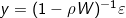 , a more compact expression for the autoregressive nature of the model. The
  factor can be thought of as a spatial autocorrelation operator with global spatial autocorrelation level ρ. All SAMs use some form of this operator to capture the spatial dependence among observations.
3. A Taxonomy of Spatial Autoregressive Model Specifications
The spatial autoregressive structure, and its characteristic factor, can be applied to the response (y), predictors (X), and error (ε) components of the traditional regression equation creating a flexible framework for analysis. The matrix multiplication of the weights matrix W with a covariate is called a spatial lag, and represents a linear combination of the values of that component and neighboring observations (as defined by the weights matrix). This multiplication expresses the spatial dependence among locations by replacing the value of a variable at a location with a spatially weighted average of its neighbors’ values. For example, if there are n locations in the study area, a spatial lag of the predictor variables is the left-multiplication of the n×n spatial weights matrix on the predictors X, which generates the n×k spatial lag WX . For the response variable y the same procedure generates a n×1 spatial lag Wy. As above, these spatially lagged terms are accompanied by parameters, ρ for lags of the response variable and γ for lags of the predictor variables, that capture the strength of the spatial autocorrelation among those observations of that variable. Often, the spatial weights matrix used during model estimation is standardized, or transformed in a way to preserve certain properties. Row standardization - ensuring the rows of W sum to 1 - is the most common of these but is not always the most preferable (see Elhorst, 2014 for details).
Applied to the error component of a regression analysis, a spatial autoregressive structure segments the error, ε, of a nonspatial regression y=Xβ+ε into two parts: a spatially autocorrelated term and a nonspatial term. To do this, the nonspatial regression is rewritten as y=Xβ+u and the error is decomposed as u=λWu+ε where λ is a parameter to be calibrated and ε is a n×1 vector of independent and identically distributed normal nonspatial errors. Estimates of the parameter λ express the average strength of spatial autocorrelation among the errors conditional on W.
The inclusion and exclusion of a spatial lagged response, spatial lagged predictors, and the spatial error decomposition define a taxonomy of SAM specifications (Fig. 1). Each combination of the lagged components defines a different SAM and different form of spatial dependence. Branching out from the classic ordinary least squares (OLS) regression (Fig. 1a), the most basic SAMs are the spatial lag of X model (SLX – Fig. 1b), and the spatial error model (SEM – Fig. 1c), and the lag model (SAR – Fig. 1d). Each of these models includes only one of the lag components presented above. The SLX model introduces the spatial lag WX of the predictors and the vector of parameters γ. The SAR model includes the spatial lag Wy of the response variable and the scalar parameter ρ. The SEM partitions the error terms and adds the scalar parameter λ.
Figure 1. Taxonomy of spatial autoregressive models. Arrows illustrate how the progressive addition of spatially lagged components to ordinary least square regression analysis increase specification complexity. Adapted from Elhorst (2014). Source: authors.
Crucially, the use of these models should be matched to a researcher's conceptualization of the spatially structured real-world process they believe to be responsible for the observed data. For example, the housing price examples presented in the motivation section can be matched to each model. If a researcher is modeling home prices and believes the price of surrounding homes affects home prices, they would select the SAR model. The SLX model would match the case where the condition of surrounding properties impacts price, and the SEM model for the case where unmeasured neighborhood reputation impacts price.
In many cases a researcher may believe that multiple spatially dependent factors shape the data generating process. To accommodate these situations, the next layer of SAMs includes multiple lagged components. The Kelejian-Prucha model (SAC – Fig. 1e) combines a spatial lag of y and the spatial error component. The Spatial Durbin model (SDM – Fig. 1f) includes spatial lags of X and y , while the spatial Durbin error model (SDEM – Fig. 1g) includes a spatial lag of X and a spatial error component. These models express increasingly complex forms of spatial dependence among the data and nest the more parsimonious SAR, SLX, and SEM models within them. Inclusion of all three spatially lagged components produces the generalized nesting spatial model (GNS). However, the GNS specification, which is similar to the Manski neighborhood effects model (Manski, 1993), is not often commonly used in empirical work for reasons presented below.
4. The Applicability and Interpretation of Spatial Autoregressive Models
There is debate as to whether several forms of SAM can be meaningfully applied to many real-world processes and how to properly interpret the relationships estimated by these models (see Pinske and Slade, 2010; Gibbons and Overman, 2012; LeSage, 2014). The debate centers on the difficult task of properly specifying the spatially dependent structures of the data generating process and how different SAMs incorporate local versus global spillover effects into the model. On the first point, in practice researchers often do not have a detailed understanding of the many interacting processes creating an observed phenomenon. If a researcher uses a SAM that models the processes too simplistically, the effects of spatial dependence may not be accounted for. Alternatively, if a researcher uses an overly complex SAM they may overfit their model. The parameter estimates of an overfitted model are not meaningful because they incorporate some of the variation in the residuals as if that variation reflected model structure (for further discussion see LeSage and Pace, 2014; Ver Hoef et al., 2018; Kedron et al., 2022).
SAM specification is further complicated by the two types of spatial dependencies or spillovers that are introduced by including different spatially lagged components in the model. Including a spatial lag of the predictor Wy into a SAM introduces a global spillover effect such that a change in a predictor X in any location will affect the response y in all other locations. This global effect exists even when the spatial weights matrix constrains spatial dependence to a subset of nearby regions. This is the case because each the response variable observed at each location affects its surrounding neighbors, which in turn affect their surrounding neighbors, and so on. These dependencies create a progressively diminishing but rippling indirect effect of the change in the predictor across the entire study area. A locally constrained version of this process occurs when WX is included in a SAM. In this case a change in the value of the predictor in one location affects that location's response variable, and those in the surrounding areas. As long as the SAM does not include a spatially lagged response variable, the ripple effects end in those neighboring regions.
Crucially, in the case of both local and global spillovers the estimated parameter values of γ and ρ associated with the spatially lagged predictor or response variables capture of both direct and indirect effects. As such these estimates cannot be interpreted as β estimates in OLS regression that indicate the change in response variable associated with a unit change in the predictor variable. Direct effects are the product of the relationship between a predictor and response variable and are interpretable like conventional OLS parameter estimates. In contrast, indirect effects are the global or local spatial spillover effects that extend beyond the direct effect and across locations. Golgher and Voss (2016) provide the derivation of each type of effect for different SAMs and discuss further how to interpret indirect effects.
Considering both the challenge of model specification and the need to differentiate direct and indirect effects, LeSage (2014) argues that the SDM and SDEM are the SAMs that best lend themselves to meaningful interpretation. As such, LeSage recommends a specification procedure rooted in a researcher's belief about whether global or local spillovers are likely driving the process under study. If a researcher believes spatial dependencies are local, they can begin with the SDEM model which will allow them to work back up the SAM taxonomy and make comparisons to more parsimonious SEM, SLX, and OLS models. If a researcher believes the spatial dependencies of the process under study are global, they can begin with the SDM model and make comparisons to SLX, SAR, and OLS models. Alternatively, the GNS is not commonly used as the starting point for applied work because it is only weakly identifiable, generating higher uncertainty in parameter estimates (Gibbons and Overman, 2012), and when identifiable may often be overparameterized (Burridge et al. 2016). Plainly, the inclusion of all possible spatial effects makes it difficult to interpret and reliably estimate any single spatial effect. As such, the GNS is not a viable alternative compared to the SDM or SDEM for the starting point of a data analysis.
5. Estimation and Implementation
5.1 Model Estimation Procedures
Spatial dependence complicates the estimation of SAM parameters as compared to a standard OLS model (Fischer and Wang, 2011). Initial computationally expensive SAM estimation techniques involved direct maximum likelihood estimation (Ord, 1975). Maximum likelihood estimation utilizes a function that describes the likelihood of a set of parameters given the data. The form of the likelihood function is determined by the specification of the SAM being fit. The fitting procedure optimizes the likelihood function using numerical optimization techniques. A SAM's estimated parameters are those that generate the highest likelihood of observing the data under a given model specification.
However, the likelihood function often takes a form that is not conducive to straightforward optimization. To circumvent these difficulties, some estimation techniques exploit aspects of the model structure for computational complexity, accuracy, and speed. These often use sparse matrix operations or quasi-likelihood functions that approximate the true likelihood function (e.g., Pace and Berry, 1997). Computational innovations in the estimation procedure have contributed to the widespread use and scalability of spatial autoregressive models in geographical and econometric research. Due to these techniques and modern computer architectures, SAMs can accept tens of thousands to hundreds of thousands of observations with little effect on the time needed to fit the models.
While modern estimation routines are sophisticated maximum likelihood methods (Kelejian and Prucha, 2007; Arraiz et al., 2010; Drukker et al., 2010), other estimation techniques have seen development in spatial autoregressive models. Among these techniques are generalized method of moments estimators (Kelejian and Prucha, 1998; Kelejian and Prucha, 1999; Lee, 2003; Lee, 2004), Bayesian approaches (LeSage and Pace, 2009), instrumental variables (Anselin, 1980), and spatial filtering methods (Griffith, 2003). More broadly, the recommended estimation technique for SAM is to begin with the generalized method of moments before proceeding to alternatives such as maximum likelihood estimation (Anselin and Rey, 2014).
5.2 Software Implementing Spatial Autoregressive Models
There are a variety of software programs capable of implementing SAMs. Open source code for SAMs can be found in the spreg package of the Python Spatial Analysis Library (PySAL; https://pysal.org/spreg/), the spatialreg package of the R-Spatial ecosystem (https://cran.r-project.org/web/packages/spatialreg/index.html), or the Spatial Econometrics Toolbox in MATLAB (https://www.spatial-econometrics.com/). Beyond the source code, GeoDa is a graphical user interface that enables a variety of spatial data analyses including spatial regression (https://geodacenter.github.io/; Anselin and Rey, 2014). These packages and interfaces offer varying levels of abstraction to users and not all provide the separate estimates of direct and indirect effects needed for model interpretation.
For more information on using SAMs in practice, a worked example of a spatial regression analysis in R using spatialreg can be found at https://walker-data.com/census-r/modeling-us-census-data.html#spatial-regression.
6. Conditional Autoregressive (CAR) Models
The hallmark feature of SAMs is that they model spatial structure simultaneously—random variables appear on both sides of the model equations. In the spatially-lagged y model (for example), the same random variable yi simultaneously appears on the left side of the ith regression equation and on the right side of the equations of neighbors of i. This paradigm (termed simultaneous autoregressive, or SAR, modeling) is the source of many of the issues of interpretation discussed in Section 4: the set of regression equations must be solved differently from a nonspatial regression to account for the simultaneously occurring variables (Smith, 2014). However, the matrix equations produced by SAR models are simple to conceptualize in the context of nonspatial regression, which has facilitated their widespread use.
Alternatively, analysts may model spatial structure conditionally, whereby the random variable y at location i is conditionally dependent on neighboring values of y (Ver Hoef et al., 2018). That is, a model is specified for the probability distribution of yi given the values of its neighbors. While this generates a more complex set of regression equations, the conditional formulation enables Bayesian inference and allows for the specification of hierarchical spatial models (Banerjee et al., 2014; Smith, 2014). The SAR and CAR models are equivalent under certain assumptions, but generally represent different ways of thinking about spatial structure and thus produce different conclusions for modelers (Cressie, 1991).
7. Concluding Remarks
Spatial autoregressive modeling is an established and flexible statistical framework that researchers can use to estimate variable relationships when observations are spatially dependent. A number of alternative SAM specifications are available to researchers, although selection among these alternatives and proper specification can be challenging. A researcher must choose what components of the regression model need to be spatially lagged and create a spatial weights matrix that identifies how spatial dependencies in those components are structured. Both choices can dramatically impact the estimates of a SAM (LeSage 2009, Harris et al. 2011). Ultimately, the use and proper specification of SAMs is the responsibility of the researcher who must choose the model form that best represents their conceptualization of the relationships and spatial dependencies relevant to the phenomena they are studying. If properly specified, SAMs can provide reliable estimates of the relationships between variables in the presence of a spatially structured data generating process.
Anselin, L. (1980). Estimation methods for spatial autoregressive structures. Regional Science Dissertation and Monograph Series, Cornell University, Ithaca, NY.
Anselin, L. (1988). Spatial Econometrics: Models and Methods. Norwell, MA: Kluwer Academic Publishers.
Anselin, L. (1989). What is Special About Spatial Data? Alternative Perspectives on Spatial Data Analysis. UC Santa Barbara NCGIA Technical Reports, 89-4.
Anselin, Luc. (2010). Thirty Years of Spatial Econometrics. Papers in Regional Science 89, (1), 3–25. https://doi.org/10.1111/j.1435-5957.2010.00279.x.
Anselin L., and Rey S.J. (2014) Modern spatial econometrics in practice: A guide to GeoDa, GeoDaSpace and PySAL. GeoDa Press LLC.
Arraiz I, Drukker D.M., Kelejian H.H., Prucha I.R. (2010). A Spatial Getis-Ord-type Model with Heteroscedastic Innovations: Small and Large Sample Results. Journal of Regional Science, 50, 592–614.
Bailey, T.C., and Gatrell, A.C. (1995). Interactive spatial data analysis. Longman Scientific & Technical, New York.
Banerjee, S., Carlin, B.P., and Gelfand, A.E. (2014). Hierarchical Modeling and Analysis for Spatial Data, 2nd edition. Chapman and Hall/CRC Press Monographs on Statistics and Applied Probability, Boca Raton, FL.
Bivand, R. (2017). Revisiting the Boston data set – Changing the units of observation affects estimated willingness to pay for clean air. Region, 4 (1), 109-127.
Burridge, P., Elhorst, J.P., and Zigova, K. (2016). Group Interactions in Research and the Use of General Nesting Spatial Models. In B.H. Batagi, J.P. LeSage, and R.K. Pace (eds.), Spatial Econometrics: Quantitative and Limited Dependent Variables (Vol. 37, 223-258). Emerald Group Publishing Limited.
Cressie, N. (1991). Statistics for Spatial Data. Wiley Series in Probability and Mathematical Statistics.
Drukker, D.M., Egger, P., and Prucha, I.R. (2010). On Two-step Estimation of a Spatial Autoregressive Model with Autoregressive Disturbances and Endogenous Regressors. Available here.
Elhorst, J. P. (2014). Linear Spatial Dependence Models for Cross-Section Data. In Spatial Econometrics, by J. Paul Elhorst, 5–36. SpringerBriefs in Regional Science. Berlin, Heidelberg: Springer Berlin Heidelberg. https://doi.org/10.1007/978-3-642-40340-8_2.
Fischer, M.M., and Wang, J. (2011). Spatial Data Analysis: Models, Methods, and Techniques. Springer.
Gibbons, S., and H. G. Overman. (2012). “Mostly Pointless Spatial Econometrics?” Journal of Regional Science 52, 2: 172–91. https://doi.org/10.1111/j.1467-9787.2012.00760.x.
Golgher, A. B., and Voss, P.R. (2016). How to Interpret the Coefficients of Spatial Models: Spillovers, Direct and Indirect Effects. Spatial Demography 4 (3), 175–205. https://doi.org/10.1007/s40980-015-0016-y.
Griffith, D.A. (2003) Spatial autocorrelation and spatial filtering: Gaining understanding through theory and scientific visualization. Springer Verlag, Berlin.
Halleck Vega, S. and Elhorst, P. (2013). On spatial econometric models, spillover effects, and W, 53rd Congress of the European Regional Science Association: "Regional Integration: Europe, the Mediterranean and the World Economy", 27-31 August 2013, Palermo, Italy, European Regional Science Association (ERSA), Louvain-la-Neuve.
Hastie, T., Tibshirani, R., and Friedman, J. (2008). The Elements of Statistical Learning: Data Mining, Inference, and Prediction, 2nd edition Springer.
Harris, R., Moffat, J., and Kravtsova, V. (2011). In Search of W. Spatial Economic Analysis 6 (3), 249–70. https://doi.org/10.1080/17421772.2011.586721.
Kedron, P., Quick, M., Hilgendorf, Z., & Sachdeva, M. (2022). Using the specification curve to teach spatial data analysis and explore geographic uncertainties. Journal of Geography in Higher Education, 46(2), 304-314.
Kelejian, H.H. and Prucha, I.R. (1998). “A Generalized Spatial Two-Stage Least Squares Procedures for Estimating a Spatial Autoregressive Model with Autoregressive Disturbances.” Journal of Real Estate Finance and Economics, 17, 99-121.
Kelejian, H.H. and Prucha, I.R. (1999). “A Generalized Moments Estimator for the Autoregressive Parameter in a Spatial Model.” International Economic Review, 40, 509-533.
Kelejian H.H., and Prucha, I.R. (2007). “HAC Estimation in a Spatial Framework.” Journal of Econometrics, 140, 131–154.
Lee, L.-F. (2003). Best spatial two-stage least squares estimators for a spatial autoregressive model with autoregressive disturbances. Econometric Reviews, 22: 307–335.
Lee, L.-F. (2004). Asymptotic distributions of quasi-maximum likelihood estimators for spatial autoregressive models. Econometrica, 72: 1899–1925.
LeSage, J.P., and Pace, R.K. Introduction to Spatial Econometrics. Chapman and Hall/CRC Press, 2009.
LeSage, J.P. (2014). What Regional Scientists Need to Know about Spatial Econometrics. The Review of Regional Studies, 44: 13-32.
LeSage, J. P., & Pace, R. K. (2014). The biggest myth in spatial econometrics. Econometrics, 2(4), 217-249.
Manski, C. F. (1993). Identification of Endogenous Social Effects: The Reflection Problem. The Review of Economic Studies, 60 (3), 531-542.
Ord, J.K. (1975) Estimation methods for models of spatial interaction. Journal of the American Statistical Association 70, 120–126.
Pace R.K., and Barry R. (1997) Quick computation of spatial autoregressive estimators. Geographical Analysis 29, 232–246.
Pinkse, J. and Slade, M.E. (2010). The future of spatial econometrics. Journal of Regional Science, 50:103–117.
Rogerson, P. (2021). Spatial Statistical Methods for Geography. SAGE Publications, Ltd..
Smith, T.E. (2014). Notebook on Spatial Data Analysis [online]. https://www.seas.upenn.edu/~tesmith/NOTEBOOK/index.html
Ver Hoef, J. M., Peterson, E. E., Hooten, M. B., Hanks, E. M., & Fortin, M. J. (2018). Spatial autoregressive models for statistical inference from ecological data. Ecological Monographs, 88(1), 36-59.
Whittle, P. (1954). On Stationary Processes in the Plane. Biometrika, 41 (3/4), 434-449.
Keywords: