DC-39 - Time-of-Arrival (TOA) Localization for Indoor GIS
Indoor geographic information system (GIS) opens up a new frontier for identifying, analyzing and solving complex problems. In many indoor GIS-driven applications such as indoor wayfinding and logistics planning and management, determination of location information deserves special attention because global positioning system (GPS) may be inaccessible. Alternative methods and systems have emerged to overcome this hurdle. The time-of-arrival (TOA) measurement is one of the most adopted metrics in numerous modern systems such as radar, acoustic/ultra-sound-based tracking, ultra-wide band (UWB) indoor localization, wireless sensor networks (WSN) and Internet of things (IoT) localization. This topic presents the TOA technique and methods to solve the localization and synchronization problem. We also introduce variants of the TOA system schemes, which are adopted by real-world applications. As a use case of the TOA technique realized in practice, a UWB localization system is introduced. Examples are given to demonstrate that indoor localization and GIS are tightly interconnected.
Author and Citation Info:
Zhao, S. and Chu, T. (2021). Time-of-Arrival (TOA) Localization for Indoor GIS. The Geographic Information Science & Technology Body of Knowledge (3rd Quarter 2021 Edition), John P. Wilson (ed.). DOI: 10.22224/gistbok/2021.3.1.
This entry was first published on July 16, 2021. No earlier editions exist.
Nowadays, location-based services (LBS) have become an integral part of our everyday life and increasing demand for LBS is driving rapid development of localization techniques for a wide spectrum of applications. In a typical outdoor environment, signals transmitted from global navigation satellite systems (GNSS) enable users to determine their real-time location and speed. However, in indoor environments such as an enclosed parking garage of a big shopping mall where we may easily get lost, GNSS signals are subject to significant attenuation or even complete blockage. To address this issue, alternative techniques have emerged as promising indoor localization solutions.
Microelectromechanical systems (MEMS) based inertial measurement units (IMU) are usually used as low-cost localization sensors. They can output high-frequency location, speed and attitude results by continuously measuring angular rates and linear accelerations. Despite their independence to the ambient environment, the cumulative errors are inevitable and grow large over time. To restrain the error accumulation in the indoor environments, MEMS-based IMU sensors usually work with light detection and ranging (Lidar) and/or visual sensors to achieve simultaneous localization and mapping (SLAM) (Vidal et al., 2018; Su et al., 2021). Although this sensor integration strategy helps slow down the cumulative position and attitude errors, the user cost of the sensors is prohibitive for most LBS users and the ambient environment is required to be highly textured for robust localization (Debeunne & Vivet, 2020).
Recent studies have also extensively investigated the potential of indoor localization by leveraging radio frequency (RF) or ultrasonic signals in various wireless communication systems such as radio-frequency identification (RFID) (El-Absi et al., 2018), radar (Zhu et al., 2018), acoustic/ultra-sound-based tracking (Zhang et al., 2017), ultra-wide band (UWB) (You et al., 2020), and wireless sensor networks (WSN) (Cheng et al., 2020). Common properties collected between signal transmitters and receivers for localization involve received signal strength (Koike-Akino et al., 2020), arrival time (He & So, 2020) or directional measurements (Hou et al., 2018).
In this topic, we aim to offer an introduction to the time-of-arrival (TOA)-based localization technique including the concept, problem formulation, solution, and implementation. Firstly, a TOA measurement model for a generalized RF signal-based indoor localization system is introduced. The optimal formulation for the TOA localization problem is then presented in the form of a weighted least squares (WLS) minimizer. After theoretical lower bound for TOA localization is explained, several methods are put forward, followed by three variants of the TOA structure that are adopted by real-world applications. Then, a UWB localization system, as an exemplary TOA technique study case, is introduced and discussed. The conclusion summarizes tight relationship between indoor localization and geographic information system (GIS).
Equipped with a number of anchor nodes (ANs) with known positions, we aim to localize a user device (UD) using RF signal communications between the UD and ANs. In our context, the TOA measurement between the UD and AN #i is obtained by recording the signal transmission and reception time stamps, which are based on the local clock sources of the transmitter and the receiver. Figure 1 shows the components of such a TOA localization system.
Figure 1. A TOA localization system. Source: authors.
A TOA measurement can be formed in two ways, i.e., an AN transmits signal and the UD receives, or vise-versa. We denote the two types of TOA measurements formed by the signal from an AN to the UD by ρ and formed by the reverse direction by τ, respectively. They are expressed as
Where represents the local time, and are the local time instants at the UD and the AN, respectively; is the reference or true time, the subscripts and represent reception and transmission, respectively; the superscripts and denote the UD and the AN, respectively. Thus, and are the respective reference reception and transmission time instants at the UD, and and are the respective reference reception and transmission time instants at the UD. In addition, and are the measurement noises that are usually independently Gaussian distributed, i.e., and .
In order to obtain the position and/or clock offset of the UD, we need to connect the TOA measurements given by and with the UD position and/or clock offset with respect to the reference time. We note that the measurements contain the true distance along with the clock offset between the UD and AN. Therefore, it is further written by
where and are the K-dimensional (K = 2 or 3) coordinates of the AN and UD, respectively, is the Euclidean norm, and are the respective clock offsets of the AN and UD with respect to the reference time, and is the signal propagation speed.
In fact, in the models of (3) and (4), we have an implicit assumption that the coordinates and the clock offsets are constant during signal propagation. This assumption holds in most cases. For example, we assume RF signal is used for communication between the UD and AN, and they have a distance of 300 m. Then the propagation time for one-time communication is only 1e-6 s. A typical oscillator that acts as the clock source for a device usually has a frequency drift at the level of ±20 parts per million (ppm) (IEEE Computer Society, 2016), which will only cause ±0.6 mm error. This is usually safe to be ignored. In addition, the clock offset of the AN is usually known by synchronization such as using round-trip communication (Shi et al., 2020).
Now, the localization (and synchronization) problem becomes finding the value of (and ) given sufficient number of TOA measurements. Figure 2 illustrates the principle of TOA localization (and synchronization) with a two-dimensional (2D) example. In this figure, R1, R2 and R3 are the true distances between the ANs and the UD, and b is the clock offset of the UD with respect to the synchronous ANs. The correct UD position is at the red spot, the intersection of the three solid line circles with the ANs as their centers. The dashed circles are generated by the TOA measurements, which include the true distances and the clock offset. Those gray intersection points of the dashed circles are caused by the common clock offset between the UD and the ANs. We have to find out the common clock offset to determine the real intersection point, which represents the actual location of the UD.
Figure 2. TOA Localication Princple. Source: authors.
We assume that there are M AN-to-UD measurements and N UD-to-AN measurements, and write the TOA measurements into the collective form as
The localization (and synchronization) problem is to find the UD position of (and the clock offset ) given the TOA measurement vector .
We denote the parameters to be estimated by . Our aim is to minimize the residuals, which are the difference of the TOA measurements and the estimated TOA values generated from the estimated parameter , in a least squares sense. The localization (and synchronization) problem can be formulated as a WLS minimizer:
is in a least squares sense, and is the inverse of the measurement noise covariance, and is the i-th element of a vector.
While the WLS minimizer is one of the most adopted formulations (Yan et al., 2013), there are also other ways to formulate the localization problem such as linearizing the problem by squaring the TOA equation and ignoring the higher order noise terms (Bancroft, 1985; Chan & Ho, 1994). In this way, some closed-form methods can be derived. However, usually far field and small noise conditions are needed, constraining the application of such methods. The minimizer given by is equivalent to a maximum likelihood (ML) estimator, which is the optimal formulation for this problem.
When we design an estimator, we are always curious about how good performance it can achieve. For the WLS minimizer described in the previous section, we also need to know its theoretical performance. The Cramér-Rao lower bound (CRLB) is a theoretical lower bound on the covariance of an unbiased estimator of a deterministic parameter. CRLB is the covariance of the parameter θ to be estimated and is equal to the inverse of the Fisher information matrix (FIM) denoted by F.
The FIM is related to the derivative of the likelihood function , i.e.,
where is the entry of a matrix at the i-th row and the j-th column, and is the expectation operator.
When the measurement noise is Gaussian distributed, the likelihood function is expressed as
where and is the matrix determinant.
Therefore, we have
The measurement noise, expressed by , is zero-mean. Therefore, . Then, we have
Our goal is to minimize the object function (6) to determine the UD position and clock offset. One straightforward idea is to find the solution by updating the estimated parameters iteratively. Let us denote the estimated parameter by . Following (Foy, 1976), we conduct the Taylor series expansion on the measurements, ignore the higher order terms, and come to
where is the collective form of all the measurement noise.
We denote the design matrix by , which has a similar form to (8) in such a localization problem, the incremental parameter by , and the residual by . Then, we rewrite (9) to .
The estimate of in the sense of weighted least squares is given by . The estimated parameter is updated iteratively by .
The above iterative method is also referred to as Gauss-Newton method. There are also some variations such as the Levenberg-Marquardt method, which has improved robustness but requires higher computational complexity. Although the iterative method is straightforward and simple to implement, it suffers from some problems. One of the drawbacks of the iterative method is that it requires a good initial guess, otherwise, it will cost more iteration times or even result in local minima. Generally, it is easier to obtain a correct solution if the initial guess is closer to the true value. However, obtaining a good initial guess is not a trivial task. Besides, the objective function (6) is nonlinear in nature due to the absolute operator and it usually has some local “valleys” or minima that can trap the iterative method.
There are extensive studies on alternative solutions for the ML-based localization (and synchronization) problem. We introduce two categories of them, i.e., the closed form method and convex optimization method.
6.1 Closed-form Method
Closed-form methods have been extensively investigated (Bancroft, 1985; Zhu & Ding, 2010; Zhao et al., 2020). A basic principle of this type of method is to convert the nonlinear problem to a linear one based on some reasonable assumptions. Here, we present a close-form method inspired by the study of Bancroft (1985) as an example. The basic idea is to employ intermediate variables, which can be linearly expressed by the processed measurements and the unknown parameters.
We denote the distance between the UD and AN #i by . For simplicity, we only consider the case that all ANs are synchronized and only one-way TOA measurements ρ are used. We ignore the propagation speed c (equivalent to converting all the unit from second to meter). The TOA measurement (3) is re-written by
.
The square of is
We re-arrange the order of the terms on both sides of the equation and come to
We denote the following symbols
Matrix , matrix , scalar , vector , and noise vector , where is the identity matrix of size K.
Then, (10) becomes ,
where is an M-element vector with all elements being 1.
We note that . Therefore, the WLS solution for is
By observing (11), we know that D is related to the UD-AN distance which is not known at this stage yet. We thereby ignore D first and obtain
,
where and .
We come to . Based on the definition of , we have . Thus, we have the following equation
The scalar variable can be obtained by solving this quadratic equation. Then the parameter vector can be estimated by the solution denoted by . The estimation parameter is given by .
This is the rough estimate of the parameter and it needs further refinement by the WLS equation (11). We need to know the matrix D. Luckily, at this stage, we have a rough estimate of . When the measurement noise is small, its square term can be ignored. We then have
, where the distance term can be estimated using .
The root mean square error (RMSE) of this closed-form method is equal to the CRLB under the condition of small measurement noise and far field. It is not exactly equivalent to the original ML problem due to ignoring high order terms of the measurement noise. But as we can see, all the steps can be solved analytically without iteration and we do not need an initial guess as required by the iterative method. These features make the closed-form method more appealing for the size and power constrained devices such as IoT systems and WSNs.
6.2 Convex Optimization
The non-convexity of the ML objective function (6) will result in more than one local minima. In many cases, it is not easy to find the global minimum as the correct position and clock offset solution. Convex optimization is to convert the original non-convex problem to a convex one through “relaxation”. However, converted convex problem is an approximation of the original problem. Therefore, compromise on performance degradation, i.e., lower accuracy, has to be made.
In this subsection, we present a convex optimization technique for a simplified case (Cheung et al., 2004), i.e., the UD is synchronized with the AN, i.e., , and only one-way TOA measurements are adopted. We first rewrite the original ML problem to a constrained minimization one as
subject to
where .
We note that for an arbitrary vector x, there is an equation that . Therefore, the objective function becomes
where .
We can see that the diagonal entries of is
, where .
We ignore the term since it is a constant and does not affect the minimizer. The original minimization problem becomes
We note that the objective function (13) and equation (14) are now convex, but the quadratic equations (15) and (16) are not convex. They are equal to
We use the semidefinite relaxation technique, i.e., drop the rank 1 constraints. Therefore, the problem is relaxed to
This is a convex problem and can be solved with established solvers such as CVX (Grant & Boyd, 2014).
We should note that the above-mentioned semidefinite programming method is an approximation to the original localization problem, and thus the solution is not optimal (Beck et al., 2008). In addition, the convex relaxation process is usually tricky and relies on one’s insights, understanding, and some luck to find a good relaxation approach.
TOA-based localization systems have a number of variants. The adoption of a particular scheme is dependent upon the requirements of the application scenario. We introduce some of the variants in this section.
7.1 One-way TOA
A popular scheme which is widely adopted in real-world applications such as the global navigation satellite systems (GNSSs) is one-way TOA (Kaplan & Hegarty, 2006). There is only one-way communication between a UD and an AN. From the measurement point of view, only ρor τis available in (5).
Figure 3 shows the two schemes for one-way TOA. The left figure is what GNSSs adopt. The UD is a receiver only to receive the broadcast signals from ANs. This makes the system support unlimited number of UDs. In addition, the UD does not need to emit any signals and thus is “silent”. This feature enables better security and privacy for the UDs. It is worth noting that in GNSS applications, the signals from ANs are simultaneously broadcast. This requires code division or frequency division to avoid air collision. Time division signal broadcast is also investigated in recent years and for low-cost devices, the clock drift during different signal transmit slots must be estimated and compensated to reduce errors (Shi et al., 2020).
The right diagram of Figure 3 has a reverse communication link compared with the left one. The UD actively transmits signals that are received by the ANs. The localization process is completed in somewhere else than the UD. Therefore, it is suitable for tracking applications such as drone navigation. Besides, it has better scalability since all the ANs are passively listening and thus hav eno limitation on numbers.
Figure 3 One-way TOA scheme. Left: The ANs transmit and the UD receives. Right: The UD transmits and the ANs receive. Source: authors.
One-way TOA scheme requires synchronization between ANs. There are generally three ways to achieve such synchronization including high accuracy clocks and control stations, cable connection in regional applications, and pair-wise wireless communications between ANs. High accuracy clock sources are usually atomic clocks such as cesium and rubidium clocks, which are usually expensive and large. Cable connection is reliable but not flexible and is difficult to maintain. Pair-wise wireless communications between ANs have better flexibility but require more temporal and/or spectral expenses.
7.2 Two-way TOA
In such a scheme, there is at least one round-trip communication between each pair of UD and AN as shown in Figure 4 (Gholami et al., 2016). An advantage of the two-way TOA scheme is that ANs are not necessarily synchronous. As an example, we assume a system in which the UD transmits first, and the ANs receive and then respond. The clock offset between the UD and each AN can be ignored if the internal turn-around time in the AN is short enough. In this case, we do not have to estimate the clock offset/drift between the UD and the ANs and we have more available TOA measurements compared with the one-way scheme. Therefore, the two-way TOA scheme has higher localization accuracy than the one-way counterpart.
Let us see the drawbacks of the two-way scheme. It requires all UD and ANs to be transceivers. This leads to added costs to the whole system and is less power efficient. Furthermore, two-way communication requires heavier air traffic, limiting the scalability of the system.
Figure 4. Two-way TOA Scheme. Source: authors.
7.3 Combination of One-way and Two-way
Another variation is to combine the one-way and two-way TOA into one scheme. Figure 5 shows such a scheme in which only one AN and the UD transmit and receive signals and other ANs only receive signals passively (Zhou et al., 2010; Zhao et al., 2021). Due to the different behaviors for different ANs, this scheme is also named as “asymmetric ranging network”. The transmitted signal from AN #1 can be used to synchronize the whole network wirelessly as well as contribute to the localization for the UD. Compared with one-way TOA, this combined scheme does not require expensive clock synchronization. Neither does it have dense communication as in two-way TOA.
Figure 5. One-way and two-way combined TOA localization system diagram. Source: authors.
In recent years, UWB technology has been widely adopted for regional localization applications. It uses very narrow impulse signal to provide high precision TOA measurements. In this sub-section, we give a UWB localization system as an implementation of the TOA-based localization principles and methods presented in the previous sections.
In this UWB system, the UD broadcasts RF signal periodically, and the ANs receive the signal and measure its TOA respectively. These TOA measurements are aggregated to a center to be processed to generate the UD position. As shown in Figure 6, the localization system is comprised of a UD, several ANs, a switcher and a central computer. When the system is in operation, the UD transmits request signal through a UWB channel and the ANs receive this request to form TOA measurements which are sent to the central computer via cable network. A network device such as a switcher or a Wi-Fi adapter is needed so that the ANs can be connected to the host computer.
We use the combined one-way and two-way TOA scheme presented in Section 7 to synchronize the ANs in this system. Specifically, we assign one AN as the primary AN, which periodically sends the sync signal with local transmission timestamp. The other ANs receive this sync signal and form its own TOA measurements by recording the transmission and reception timestamps. These timestamps are filtered to suppress measurement noise. Given the positions of ANs, the clock offsets between the primary AN and other ANs can be computed. With this clock offset information, all ANs are synchronized.
When the UD transmits request signal, all ANs receive it to form the TOA measurements by subtracting the transmission time from the reception time. Another way is to form the time-difference-of-arrival (TDOA) measurements by subtracting the designated reception timestamp from all other reception timestamps. When using TDOA, the UD does not have to send its transmission timestamp so the airtime of the request signal can be shortened. All the TOA or TDOA measurements are sent to a central computer for localization computation (Zhao et al., 2017).
Based on current available UWB technologies, the reception timestamp can be precise at the level of sub-nanosecond, corresponding to about 10 cm noise on the TOA measurements. With proper algorithm design and system implementation, the standard deviation of the final location fix can be better than 5 cm (1-sigma). However, there are still some other error sources that need to be compensated such as the hardware processing delay, the antenna phase center error and the isotropy of the antenna pattern, which will all result in localization errors.
In the United States, people spend nearly 87% of time indoors on average (Klepeis et al., 2001) and therefore extending GIS from outdoor space to indoor domains is considered a matter of course. Indoor GIS leverages knowledge acquired from building information modeling (BIM), floor plans, site scans and other data sources to create 2D or three-dimensional (3D) digital indoor maps and perform geospatial analyses. Nowadays, indoor localization has deeply connected with indoor GIS to support freight logistics, emergency management, public health, and other types of applications. During an emergency evacuation, accurate indoor localization is a crucial first step for safety and security, particularly when an evacuee is in an unfamiliar facility. And indoor GIS may significantly enhance the evacuee’s situational awareness by providing the nearest and fastest exit route together with locations of potential safety risks along the route. As another example, studies have demonstrated that social distancing and contact tracing are effective measures in response to the spread of coronavirus disease 2019 (COVID-19) (Marcel et al., 2020; Lewnard & Lo, 2020). Indoor localization can help remind people of maintaining social distancing in large public facilities such as in grocery stores, fitness centers and museums. Going one step further, if an individual has been determined exposed to COVID-19, GIS can help create, analyze and visualize his/her spatio-temporal trajectory data and trace people who has been in close contact with him/her. Indoor localization along with GIS will significantly advance the current state of contact tracing, which is usually based on outdoor spaces. They are also anticipated to be helpful for studying airborne transmission of COVID-19 indoors. Leading companies such as Google, Apple and ESRI have realized the importance of indoor maps and provide corresponding programs that enable analysis, management and visualization of location data on indoor maps to support decision-making processes. Moving forward, with the rapid evolution of positioning, mobile computing and sensor technologies, indoor localization is anticipated to be more tightly coupled with GIS in miniaturized mobile devices such as smartphones to serve the needs of general public. On the other hand, as acquisition and sharing of location and map data are getting easier than ever, location privacy and public safety concerns may escalate and push for ethical and legal moves.
References:
Bancroft, S. (1985). An algebraic solution of the GPS equations. IEEE transactions on Aerospace and Electronic Systems, AES-21(1), 56-59. DOI: 10.1109/TAES.1985.310538.
Beck, A., Stoica, P., & Li, J. (2008). Exact and approximate solutions of source localization problems. IEEE Transactions on Signal Processing, 56(5), 1770-1778. DOI: 10.1109/TSP.2007.909342.
Chan, Y. T., & Ho, K. C. (1994). A simple and efficient estimator for hyperbolic location. IEEE Transactions on Signal Processing, 42(8), 1905-1915. DOI: 10.1109/78.301830.
Cheng, L., Li, Y., Xue, M., & Wang, Y. (2020). An indoor localization algorithm based on modified joint probabilistic data association for wireless sensor network. IEEE Transactions on Industrial Informatics, 17(1), 63-72. DOI: 10.1109/TII.2020.2979690.
Cheung, K. W., Ma, W. K., & So, H. C. (2004, May). Accurate approximation algorithm for TOA-based maximum likelihood mobile location using semidefinite programming. In Proceedings of the2004 IEEE International Conference on Acoustics, Speech, and Signal Processing (pp. 145-148).
Debeunne, C., & Vivet, D. (2020). A review of visual-LiDAR fusion based simultaneous localization and mapping. Sensors, 20(7), p.2068. DOI: 10.3390/s20072068.
El-Absi, M., Abbas, A. A., Abuelhaija, A., Zheng, F., Solbach, K., & Kaiser, T. (2018). High-accuracy indoor localization based on chipless RFID systems at THz band. IEEE access, 6, 54355-54368. DOI: 10.1109/ACCESS.2018.2871960.
Foy, W. H. (1976). Position-location solutions by Taylor-series estimation. IEEE Transactions on Aerospace and Electronic Systems, AES-12(2), 187-194. DOI: 10.1109/TAES.1976.308294.
Gholami, M. R., Gezici, S., & Ström, E. G. (2016). TW-TOA based positioning in the presence of clock imperfections. Digital Signal Processing, 59, 19-30. DOI: 10.1016/j.dsp.2016.07.023.
Grant, M., & Boyd, S. (2014). CVX: Matlab software for disciplined convex programming, version 2.1.
He, J., & So, H. C. (2020). A hybrid TDOA-Fingerprinting-Based localization system for LTE network. IEEE Sensors Journal, 20(22), 13653-13665. DOI: 10.1109/JSEN.2020.3004179.
Hou, Y., Yang, X., & Abbasi, Q. H. (2018). Efficient AoA-based wireless indoor localization for hospital outpatients using mobile devices. Sensors, 18(11), p.3698. DOI: 10.3390/s18113698.
IEEE Computer Society. (2016). IEEE standard for low-rate wireless networks. IEEE Std 802.15.4-2015 (Revision of IEEE Std 802.15.4- 2011).
Kaplan, E., & Hegarty, C. (2006). Understanding GPS: principles and applications (second edition). Norwood MA: Artech House.
Klepeis, N. E., Nelson, W. C., Ott, W. R., Robinson, J. P., Tsang, A. M., Switzer, P., Behar, J.V., Hern, S.C., & Engelmann, W. H. (2001). The National Human Activity Pattern Survey (NHAPS): a resource for assessing exposure to environmental pollutants. Journal of Exposure Science & Environmental Epidemiology, 11(3), 231-252. DOI: 10.1038/sj.jea.7500165.
Koike-Akino, T., Wang, P., Pajovic, M., Sun, H., & Orlik, P. V., 2020. Fingerprinting-based indoor localization with commercial MMWave WiFi: A deep learning approach. IEEE Access, 8, 84879-84892. DOI: 10.1109/ACCESS.2020.2991129.
Marcel, S., Christian, A., Richard, N., Silvia, S., Emma, H., Jacques, F., Marcel, Z., Gabriela, S., Manuel, B., Annelies, W., Isabella, E., Matthias, E., & Nicola, L. (2020). COVID-19 epidemic in Switzerland: on the importance of testing, contact tracing and isolation. Swiss Medical Weekly, 150(1112). DOI: 10.4414/smw.2020.20225.
Lewnard, J. A., & Lo, N. C. (2020). Scientific and ethical basis for social-distancing interventions against COVID-19. The Lancet Infectious Diseases, 20(6), 631-633. DOI: 10.1016/S1473-3099(20)30190-0.
Shi, Q., Cui, X., Zhao, S., Xu, S., & Lu, M. (2020). BLAS: Broadcast relative localization and clock synchronization for dynamic dense multi-agent systems. IEEE Transactions on Aerospace and Electronic Systems, 56(5), 3822-3839. DOI: 10.1109/TAES.2020.2979640.
Su, Y., Wang, T., Shao, S., Yao, C., & Wang, Z. (2021). GR-LOAM: LiDAR-based sensor fusion SLAM for ground robots on complex terrain. Robotics and Autonomous Systems, 140, p.103759. DOI: 10.1016/j.robot.2021.103759.
Vidal, A. R., Rebecq, H., Horstschaefer, T., & Scaramuzza, D. (2018). Ultimate SLAM? Combining events, images, and IMU for robust visual SLAM in HDR and high-speed scenarios. IEEE Robotics and Automation Letters, 3(2), 994-1001. DOI: 10.1109/LRA.2018.2793357.
Yan, J., Tiberius, C. C., Janssen, G. J., Teunissen, P. J., & Bellusci, G. (2013). Review of range-based positioning algorithms. IEEE Aerospace and Electronic Systems Magazine, 28(8), 2-27. DOI: 10.1109/MAES.2013.6575420.
You, W., Li, F., Liao, L., & Huang, M. (2020). Data fusion of UWB and IMU based on unscented Kalman filter for indoor localization of Quadrotor UAV. IEEE Access, 8, 64971-64981. DOI: 10.1109/ACCESS.2020.2985053.
Zhang, L., Huang, D., Wang, X., Schindelhauer, C., & Wang, Z. (2017). Acoustic NLOS identification using acoustic channel characteristics for smartphone indoor localization. Sensors, 17(4), p.727. DOI: 10.3390/s17040727.
Zhao, S., Cui, X., Ma, T., Jia, M., Xu, S., & Lu, M. (2017, September). Design and implementation of a wireless time synchronization based positioning system. In Proceedings of the 30th International Technical Meeting of the Satellite Division of The Institute of Navigation (ION GNSS+ 2017) (pp. 767-772).
Zhao, S., Zhang, X. P., Cui, X., & Lu, M. (2020). A closed-form localization method utilizing pseudorange measurements from two non-synchronized positioning systems. IEEE Internet of Things Journal. 8(2), 1082-1094. DOI: 10.1109/JIOT.2020.3010479.
Zhou, Y., Law, C. L., Guan, Y. L., & Chin, F. (2010). Indoor elliptical localization based on asynchronous UWB range measurement. IEEE Transactions on Instrumentation and Measurement, 60(1), 248-257. DOI: 10.1109/TIM.2010.2049185.
Zhao, S., Zhang, X. -P., Cui, X., & Lu, M. (2021). A new TOA localization and synchronization system with virtually synchronized periodic asymmetric ranging network. IEEE Internet of Things Journal, DOI: 10.1109/JIOT.2021.3055677.
Zhu, A., Qi, X., Fan, T., Gu, Z., Lv, Q., Ye, D., Huangfu, J., Sun, Y., Zhu, W., & Ran, L. (2018). Indoor localization for passive moving objects based on a redundant SIMO radar sensor. IEEE Journal on Emerging and Selected Topics in Circuits and Systems, 8(2), 271-279. DOI: 10.1109/JETCAS.2018.2798584.
Zhu, S., & Ding, Z. (2010). Joint synchronization and localization using TOAs: A linearization based WLS solution. IEEE Journal on Selected Areas in Communications, 28(7), 1017-1025. DOI: 10.1109/JSAC.2010.100906.
Learning Objectives:
Define the concept of TOA measurements, and what information is in TOA measurements.
Explain the basic framework to extract position and timing information from TOA measurements.
Summarize the theoretical bound for TOA localization.
Explain at least one method to solve the TOA localization problem.
Describe how a TOA system works via simulation and experiment.
Instructional Assessment Questions:
What are typical scenarios in which TOA localization can be used as opposed to GNSS?
List at least two names of real-world TOA localization systems.
How are TOA measurements most commonly obtained? Are there any other ways?

Indoor geographic information system (GIS) opens up a new frontier for identifying, analyzing and solving complex problems. In many indoor GIS-driven applications such as indoor wayfinding and logistics planning and management, determination of location information deserves special attention because global positioning system (GPS) may be inaccessible. Alternative methods and systems have emerged to overcome this hurdle. The time-of-arrival (TOA) measurement is one of the most adopted metrics in numerous modern systems such as radar, acoustic/ultra-sound-based tracking, ultra-wide band (UWB) indoor localization, wireless sensor networks (WSN) and Internet of things (IoT) localization. This topic presents the TOA technique and methods to solve the localization and synchronization problem. We also introduce variants of the TOA system schemes, which are adopted by real-world applications. As a use case of the TOA technique realized in practice, a UWB localization system is introduced. Examples are given to demonstrate that indoor localization and GIS are tightly interconnected.
Zhao, S. and Chu, T. (2021). Time-of-Arrival (TOA) Localization for Indoor GIS. The Geographic Information Science & Technology Body of Knowledge (3rd Quarter 2021 Edition), John P. Wilson (ed.). DOI: 10.22224/gistbok/2021.3.1.
This entry was first published on July 16, 2021. No earlier editions exist.
1. Overview
Nowadays, location-based services (LBS) have become an integral part of our everyday life and increasing demand for LBS is driving rapid development of localization techniques for a wide spectrum of applications. In a typical outdoor environment, signals transmitted from global navigation satellite systems (GNSS) enable users to determine their real-time location and speed. However, in indoor environments such as an enclosed parking garage of a big shopping mall where we may easily get lost, GNSS signals are subject to significant attenuation or even complete blockage. To address this issue, alternative techniques have emerged as promising indoor localization solutions.
Microelectromechanical systems (MEMS) based inertial measurement units (IMU) are usually used as low-cost localization sensors. They can output high-frequency location, speed and attitude results by continuously measuring angular rates and linear accelerations. Despite their independence to the ambient environment, the cumulative errors are inevitable and grow large over time. To restrain the error accumulation in the indoor environments, MEMS-based IMU sensors usually work with light detection and ranging (Lidar) and/or visual sensors to achieve simultaneous localization and mapping (SLAM) (Vidal et al., 2018; Su et al., 2021). Although this sensor integration strategy helps slow down the cumulative position and attitude errors, the user cost of the sensors is prohibitive for most LBS users and the ambient environment is required to be highly textured for robust localization (Debeunne & Vivet, 2020).
Recent studies have also extensively investigated the potential of indoor localization by leveraging radio frequency (RF) or ultrasonic signals in various wireless communication systems such as radio-frequency identification (RFID) (El-Absi et al., 2018), radar (Zhu et al., 2018), acoustic/ultra-sound-based tracking (Zhang et al., 2017), ultra-wide band (UWB) (You et al., 2020), and wireless sensor networks (WSN) (Cheng et al., 2020). Common properties collected between signal transmitters and receivers for localization involve received signal strength (Koike-Akino et al., 2020), arrival time (He & So, 2020) or directional measurements (Hou et al., 2018).
In this topic, we aim to offer an introduction to the time-of-arrival (TOA)-based localization technique including the concept, problem formulation, solution, and implementation. Firstly, a TOA measurement model for a generalized RF signal-based indoor localization system is introduced. The optimal formulation for the TOA localization problem is then presented in the form of a weighted least squares (WLS) minimizer. After theoretical lower bound for TOA localization is explained, several methods are put forward, followed by three variants of the TOA structure that are adopted by real-world applications. Then, a UWB localization system, as an exemplary TOA technique study case, is introduced and discussed. The conclusion summarizes tight relationship between indoor localization and geographic information system (GIS).
2. TOA Measurement Model
Equipped with a number of anchor nodes (ANs) with known positions, we aim to localize a user device (UD) using RF signal communications between the UD and ANs. In our context, the TOA measurement between the UD and AN #i is obtained by recording the signal transmission and reception time stamps, which are based on the local clock sources of the transmitter and the receiver. Figure 1 shows the components of such a TOA localization system.
Figure 1. A TOA localization system. Source: authors.
A TOA measurement can be formed in two ways, i.e., an AN transmits signal and the UD receives, or vise-versa. We denote the two types of TOA measurements formed by the signal from an AN to the UD by ρ and formed by the reverse direction by τ, respectively. They are expressed as
Where represents the local time,
  and
and  are the local time instants at the UD and the AN, respectively;
  is the reference or true time, the subscripts
  and
and  represent reception and transmission, respectively; the superscripts
  and
and  denote the UD and the AN, respectively. Thus,
  and
and  are the respective reference reception and transmission time instants at the UD, and
  and
and  are the respective reference reception and transmission time instants at the UD. In addition,
  and
and  are the measurement noises that are usually independently Gaussian distributed, i.e.,
  and
and  .
.
In order to obtain the position and/or clock offset of the UD, we need to connect the TOA measurements given by and with the UD position and/or clock offset with respect to the reference time. We note that the measurements contain the true distance along with the clock offset between the UD and AN. Therefore, it is further written by
where and
and  are the K-dimensional (K = 2 or 3) coordinates of the AN and UD, respectively,
  is the Euclidean norm,
  and
and  are the respective clock offsets of the AN and UD with respect to the reference time, and
  is the signal propagation speed.
In fact, in the models of (3) and (4), we have an implicit assumption that the coordinates and the clock offsets are constant during signal propagation. This assumption holds in most cases. For example, we assume RF signal is used for communication between the UD and AN, and they have a distance of 300 m. Then the propagation time for one-time communication is only 1e-6 s. A typical oscillator that acts as the clock source for a device usually has a frequency drift at the level of ±20 parts per million (ppm) (IEEE Computer Society, 2016), which will only cause ±0.6 mm error. This is usually safe to be ignored. In addition, the clock offset of the AN is usually known by synchronization such as using round-trip communication (Shi et al., 2020).
Now, the localization (and synchronization) problem becomes finding the value of (and
(and  ) given sufficient number of TOA measurements. Figure 2 illustrates the principle of TOA localization (and synchronization) with a two-dimensional (2D) example. In this figure, R1, R2 and R3 are the true distances between the ANs and the UD, and b is the clock offset of the UD with respect to the synchronous ANs. The correct UD position is at the red spot, the intersection of the three solid line circles with the ANs as their centers. The dashed circles are generated by the TOA measurements, which include the true distances and the clock offset. Those gray intersection points of the dashed circles are caused by the common clock offset between the UD and the ANs. We have to find out the common clock offset to determine the real intersection point, which represents the actual location of the UD.
Figure 2. TOA Localication Princple. Source: authors.
3. Weighted Least Squares Minimizer
We assume that there are M AN-to-UD measurements and N UD-to-AN measurements, and write the TOA measurements into the collective form as
The localization (and synchronization) problem is to find the UD position of (and the clock offset
  ) given the TOA measurement vector
  .
.
We denote the parameters to be estimated by![\boldsymbol{\theta} = [\textbf{\textit{p}}_U^T \ b_U]^T](https://latex.codecogs.com/gif.latex?%5Cboldsymbol%7B%5Ctheta%7D%20%3D%20%5B%5Ctextbf%7B%5Ctextit%7Bp%7D%7D_U%5ET%20%5C%20b_U%5D%5ET) . Our aim is to minimize the residuals, which are the difference of the TOA measurements
. Our aim is to minimize the residuals, which are the difference of the TOA measurements  and the estimated TOA values generated from the estimated parameter
  , in a least squares sense. The localization (and synchronization) problem can be formulated as a WLS minimizer:
While the WLS minimizer is one of the most adopted formulations (Yan et al., 2013), there are also other ways to formulate the localization problem such as linearizing the problem by squaring the TOA equation and ignoring the higher order noise terms (Bancroft, 1985; Chan & Ho, 1994). In this way, some closed-form methods can be derived. However, usually far field and small noise conditions are needed, constraining the application of such methods. The minimizer given by is equivalent to a maximum likelihood (ML) estimator, which is the optimal formulation for this problem.
4. Theoretical Lower Bound
When we design an estimator, we are always curious about how good performance it can achieve. For the WLS minimizer described in the previous section, we also need to know its theoretical performance. The Cramér-Rao lower bound (CRLB) is a theoretical lower bound on the covariance of an unbiased estimator of a deterministic parameter. CRLB is the covariance of the parameter θ to be estimated and is equal to the inverse of the Fisher information matrix (FIM) denoted by F.
The FIM is related to the derivative of the likelihood function , i.e.,
where![[\cdot]_{i,j}](https://latex.codecogs.com/gif.latex?%5B%5Ccdot%5D_%7Bi%2Cj%7D) is the entry of a matrix at the i-th row and the j-th column, and
is the entry of a matrix at the i-th row and the j-th column, and ![E[\cdot]](https://latex.codecogs.com/gif.latex?E%5B%5Ccdot%5D) is the expectation operator.
is the expectation operator.
When the measurement noise is Gaussian distributed, the likelihood function is expressed as
where and
and  is the matrix determinant.
Therefore, we have
The measurement noise, expressed by , is zero-mean. Therefore,
 ![E[g(\boldsymbol{\theta})^T\textbf{\textit{W}}\frac{\partial^2f(\boldsymbol{\theta})}{\partial\boldsymbol{\theta}\partial\boldsymbol{\theta}^T}] = 0](https://latex.codecogs.com/gif.latex?E%5Bg%28%5Cboldsymbol%7B%5Ctheta%7D%29%5ET%5Ctextbf%7B%5Ctextit%7BW%7D%7D%5Cfrac%7B%5Cpartial%5E2f%28%5Cboldsymbol%7B%5Ctheta%7D%29%7D%7B%5Cpartial%5Cboldsymbol%7B%5Ctheta%7D%5Cpartial%5Cboldsymbol%7B%5Ctheta%7D%5ET%7D%5D%20%3D%200) . Then, we have
. Then, we have
5. Iterative Method for the ML TOA Localization Problem
Our goal is to minimize the object function (6) to determine the UD position and clock offset. One straightforward idea is to find the solution by updating the estimated parameters iteratively. Let us denote the estimated parameter by . Following (Foy, 1976), we conduct the Taylor series expansion on the measurements, ignore the higher order terms, and come to
where is the collective form of all the measurement noise.
We denote the design matrix by , which has a similar form to (8) in such a localization problem, the incremental parameter by
  , and the residual by
  . Then, we rewrite (9) to
  .
.
The estimate of in the sense of weighted least squares is given by
  . The estimated parameter is updated iteratively by
  .
.
The above iterative method is also referred to as Gauss-Newton method. There are also some variations such as the Levenberg-Marquardt method, which has improved robustness but requires higher computational complexity. Although the iterative method is straightforward and simple to implement, it suffers from some problems. One of the drawbacks of the iterative method is that it requires a good initial guess, otherwise, it will cost more iteration times or even result in local minima. Generally, it is easier to obtain a correct solution if the initial guess is closer to the true value. However, obtaining a good initial guess is not a trivial task. Besides, the objective function (6) is nonlinear in nature due to the absolute operator and it usually has some local “valleys” or minima that can trap the iterative method.
6. Approximate Solutions for the ML TOA Localization Problem
There are extensive studies on alternative solutions for the ML-based localization (and synchronization) problem. We introduce two categories of them, i.e., the closed form method and convex optimization method.
6.1 Closed-form Method
Closed-form methods have been extensively investigated (Bancroft, 1985; Zhu & Ding, 2010; Zhao et al., 2020). A basic principle of this type of method is to convert the nonlinear problem to a linear one based on some reasonable assumptions. Here, we present a close-form method inspired by the study of Bancroft (1985) as an example. The basic idea is to employ intermediate variables, which can be linearly expressed by the processed measurements and the unknown parameters.
We denote the distance between the UD and AN #i by . For simplicity, we only consider the case that all ANs are synchronized and only one-way TOA measurements ρ are used. We ignore the propagation speed c (equivalent to converting all the unit from second to meter). The TOA measurement (3) is re-written by
The square of is
is
We re-arrange the order of the terms on both sides of the equation and come to
We denote the following symbols
Matrix , matrix
 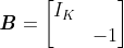 , scalar
 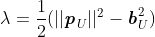 , vector
 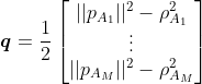 , and noise vector
  , where
  is the identity matrix of size K.
Then, (10) becomes ,
,
where is an M-element vector with all elements being 1.
We note that . Therefore, the WLS solution for
  is
is
By observing (11), we know that D is related to the UD-AN distance which is not known at this stage yet. We thereby ignore D first and obtain
where and
and  .
.
We come to . Based on the definition of
  , we have
  . Thus, we have the following equation
The scalar variable can be obtained by solving this quadratic equation. Then the parameter vector can be estimated by the solution denoted by
  . The estimation parameter is given by
  .
.
This is the rough estimate of the parameter and it needs further refinement by the WLS equation (11). We need to know the matrix D. Luckily, at this stage, we have a rough estimate of . When the measurement noise is small, its square term can be ignored. We then have
The root mean square error (RMSE) of this closed-form method is equal to the CRLB under the condition of small measurement noise and far field. It is not exactly equivalent to the original ML problem due to ignoring high order terms of the measurement noise. But as we can see, all the steps can be solved analytically without iteration and we do not need an initial guess as required by the iterative method. These features make the closed-form method more appealing for the size and power constrained devices such as IoT systems and WSNs.
6.2 Convex Optimization
The non-convexity of the ML objective function (6) will result in more than one local minima. In many cases, it is not easy to find the global minimum as the correct position and clock offset solution. Convex optimization is to convert the original non-convex problem to a convex one through “relaxation”. However, converted convex problem is an approximation of the original problem. Therefore, compromise on performance degradation, i.e., lower accuracy, has to be made.
In this subsection, we present a convex optimization technique for a simplified case (Cheung et al., 2004), i.e., the UD is synchronized with the AN, i.e., , and only one-way TOA measurements
 ![\boldsymbol{\rho} = [\rho_1 ... \rho_M]^T](https://latex.codecogs.com/gif.latex?%5Cboldsymbol%7B%5Crho%7D%20%3D%20%5B%5Crho_1%20...%20%5Crho_M%5D%5ET) are adopted. We first rewrite the original ML problem to a constrained minimization one as
are adopted. We first rewrite the original ML problem to a constrained minimization one as
subject to
where![\textbf{\textit{d}} = [d_1 \dots d_M]^T](https://latex.codecogs.com/gif.latex?%5Ctextbf%7B%5Ctextit%7Bd%7D%7D%20%3D%20%5Bd_1%20%5Cdots%20d_M%5D%5ET) .
.
We note that for an arbitrary vector x, there is an equation that . Therefore, the objective function becomes
where .
.
We can see that the diagonal entries of is
is
We ignore the term since it is a constant and does not affect the minimizer. The original minimization problem becomes
We note that the objective function (13) and equation (14) are now convex, but the quadratic equations (15) and (16) are not convex. They are equal to
We use the semidefinite relaxation technique, i.e., drop the rank 1 constraints. Therefore, the problem is relaxed to
This is a convex problem and can be solved with established solvers such as CVX (Grant & Boyd, 2014).
We should note that the above-mentioned semidefinite programming method is an approximation to the original localization problem, and thus the solution is not optimal (Beck et al., 2008). In addition, the convex relaxation process is usually tricky and relies on one’s insights, understanding, and some luck to find a good relaxation approach.
7. Variants of System Structure
TOA-based localization systems have a number of variants. The adoption of a particular scheme is dependent upon the requirements of the application scenario. We introduce some of the variants in this section.
7.1 One-way TOA
A popular scheme which is widely adopted in real-world applications such as the global navigation satellite systems (GNSSs) is one-way TOA (Kaplan & Hegarty, 2006). There is only one-way communication between a UD and an AN. From the measurement point of view, only ρ or τ is available in (5).
Figure 3 shows the two schemes for one-way TOA. The left figure is what GNSSs adopt. The UD is a receiver only to receive the broadcast signals from ANs. This makes the system support unlimited number of UDs. In addition, the UD does not need to emit any signals and thus is “silent”. This feature enables better security and privacy for the UDs. It is worth noting that in GNSS applications, the signals from ANs are simultaneously broadcast. This requires code division or frequency division to avoid air collision. Time division signal broadcast is also investigated in recent years and for low-cost devices, the clock drift during different signal transmit slots must be estimated and compensated to reduce errors (Shi et al., 2020).
The right diagram of Figure 3 has a reverse communication link compared with the left one. The UD actively transmits signals that are received by the ANs. The localization process is completed in somewhere else than the UD. Therefore, it is suitable for tracking applications such as drone navigation. Besides, it has better scalability since all the ANs are passively listening and thus hav eno limitation on numbers.
Figure 3 One-way TOA scheme. Left: The ANs transmit and the UD receives. Right: The UD transmits and the ANs receive. Source: authors.
One-way TOA scheme requires synchronization between ANs. There are generally three ways to achieve such synchronization including high accuracy clocks and control stations, cable connection in regional applications, and pair-wise wireless communications between ANs. High accuracy clock sources are usually atomic clocks such as cesium and rubidium clocks, which are usually expensive and large. Cable connection is reliable but not flexible and is difficult to maintain. Pair-wise wireless communications between ANs have better flexibility but require more temporal and/or spectral expenses.
7.2 Two-way TOA
In such a scheme, there is at least one round-trip communication between each pair of UD and AN as shown in Figure 4 (Gholami et al., 2016). An advantage of the two-way TOA scheme is that ANs are not necessarily synchronous. As an example, we assume a system in which the UD transmits first, and the ANs receive and then respond. The clock offset between the UD and each AN can be ignored if the internal turn-around time in the AN is short enough. In this case, we do not have to estimate the clock offset/drift between the UD and the ANs and we have more available TOA measurements compared with the one-way scheme. Therefore, the two-way TOA scheme has higher localization accuracy than the one-way counterpart.
Let us see the drawbacks of the two-way scheme. It requires all UD and ANs to be transceivers. This leads to added costs to the whole system and is less power efficient. Furthermore, two-way communication requires heavier air traffic, limiting the scalability of the system.
Figure 4. Two-way TOA Scheme. Source: authors.
7.3 Combination of One-way and Two-way
Another variation is to combine the one-way and two-way TOA into one scheme. Figure 5 shows such a scheme in which only one AN and the UD transmit and receive signals and other ANs only receive signals passively (Zhou et al., 2010; Zhao et al., 2021). Due to the different behaviors for different ANs, this scheme is also named as “asymmetric ranging network”. The transmitted signal from AN #1 can be used to synchronize the whole network wirelessly as well as contribute to the localization for the UD. Compared with one-way TOA, this combined scheme does not require expensive clock synchronization. Neither does it have dense communication as in two-way TOA.
Figure 5. One-way and two-way combined TOA localization system diagram. Source: authors.
8. Ultra-wide Band (UWB) Localization Systems
In recent years, UWB technology has been widely adopted for regional localization applications. It uses very narrow impulse signal to provide high precision TOA measurements. In this sub-section, we give a UWB localization system as an implementation of the TOA-based localization principles and methods presented in the previous sections.
In this UWB system, the UD broadcasts RF signal periodically, and the ANs receive the signal and measure its TOA respectively. These TOA measurements are aggregated to a center to be processed to generate the UD position. As shown in Figure 6, the localization system is comprised of a UD, several ANs, a switcher and a central computer. When the system is in operation, the UD transmits request signal through a UWB channel and the ANs receive this request to form TOA measurements which are sent to the central computer via cable network. A network device such as a switcher or a Wi-Fi adapter is needed so that the ANs can be connected to the host computer.
Figure 6. UWB Localicalization System. Source: authors.
We use the combined one-way and two-way TOA scheme presented in Section 7 to synchronize the ANs in this system. Specifically, we assign one AN as the primary AN, which periodically sends the sync signal with local transmission timestamp. The other ANs receive this sync signal and form its own TOA measurements by recording the transmission and reception timestamps. These timestamps are filtered to suppress measurement noise. Given the positions of ANs, the clock offsets between the primary AN and other ANs can be computed. With this clock offset information, all ANs are synchronized.
When the UD transmits request signal, all ANs receive it to form the TOA measurements by subtracting the transmission time from the reception time. Another way is to form the time-difference-of-arrival (TDOA) measurements by subtracting the designated reception timestamp from all other reception timestamps. When using TDOA, the UD does not have to send its transmission timestamp so the airtime of the request signal can be shortened. All the TOA or TDOA measurements are sent to a central computer for localization computation (Zhao et al., 2017).
Based on current available UWB technologies, the reception timestamp can be precise at the level of sub-nanosecond, corresponding to about 10 cm noise on the TOA measurements. With proper algorithm design and system implementation, the standard deviation of the final location fix can be better than 5 cm (1-sigma). However, there are still some other error sources that need to be compensated such as the hardware processing delay, the antenna phase center error and the isotropy of the antenna pattern, which will all result in localization errors.
9. Indoor Localization and GIS
In the United States, people spend nearly 87% of time indoors on average (Klepeis et al., 2001) and therefore extending GIS from outdoor space to indoor domains is considered a matter of course. Indoor GIS leverages knowledge acquired from building information modeling (BIM), floor plans, site scans and other data sources to create 2D or three-dimensional (3D) digital indoor maps and perform geospatial analyses. Nowadays, indoor localization has deeply connected with indoor GIS to support freight logistics, emergency management, public health, and other types of applications. During an emergency evacuation, accurate indoor localization is a crucial first step for safety and security, particularly when an evacuee is in an unfamiliar facility. And indoor GIS may significantly enhance the evacuee’s situational awareness by providing the nearest and fastest exit route together with locations of potential safety risks along the route. As another example, studies have demonstrated that social distancing and contact tracing are effective measures in response to the spread of coronavirus disease 2019 (COVID-19) (Marcel et al., 2020; Lewnard & Lo, 2020). Indoor localization can help remind people of maintaining social distancing in large public facilities such as in grocery stores, fitness centers and museums. Going one step further, if an individual has been determined exposed to COVID-19, GIS can help create, analyze and visualize his/her spatio-temporal trajectory data and trace people who has been in close contact with him/her. Indoor localization along with GIS will significantly advance the current state of contact tracing, which is usually based on outdoor spaces. They are also anticipated to be helpful for studying airborne transmission of COVID-19 indoors. Leading companies such as Google, Apple and ESRI have realized the importance of indoor maps and provide corresponding programs that enable analysis, management and visualization of location data on indoor maps to support decision-making processes. Moving forward, with the rapid evolution of positioning, mobile computing and sensor technologies, indoor localization is anticipated to be more tightly coupled with GIS in miniaturized mobile devices such as smartphones to serve the needs of general public. On the other hand, as acquisition and sharing of location and map data are getting easier than ever, location privacy and public safety concerns may escalate and push for ethical and legal moves.
Bancroft, S. (1985). An algebraic solution of the GPS equations. IEEE transactions on Aerospace and Electronic Systems, AES-21(1), 56-59. DOI: 10.1109/TAES.1985.310538.
Beck, A., Stoica, P., & Li, J. (2008). Exact and approximate solutions of source localization problems. IEEE Transactions on Signal Processing, 56(5), 1770-1778. DOI: 10.1109/TSP.2007.909342.
Chan, Y. T., & Ho, K. C. (1994). A simple and efficient estimator for hyperbolic location. IEEE Transactions on Signal Processing, 42(8), 1905-1915. DOI: 10.1109/78.301830.
Cheng, L., Li, Y., Xue, M., & Wang, Y. (2020). An indoor localization algorithm based on modified joint probabilistic data association for wireless sensor network. IEEE Transactions on Industrial Informatics, 17(1), 63-72. DOI: 10.1109/TII.2020.2979690.
Cheung, K. W., Ma, W. K., & So, H. C. (2004, May). Accurate approximation algorithm for TOA-based maximum likelihood mobile location using semidefinite programming. In Proceedings of the 2004 IEEE International Conference on Acoustics, Speech, and Signal Processing (pp. 145-148).
Debeunne, C., & Vivet, D. (2020). A review of visual-LiDAR fusion based simultaneous localization and mapping. Sensors, 20(7), p.2068. DOI: 10.3390/s20072068.
El-Absi, M., Abbas, A. A., Abuelhaija, A., Zheng, F., Solbach, K., & Kaiser, T. (2018). High-accuracy indoor localization based on chipless RFID systems at THz band. IEEE access, 6, 54355-54368. DOI: 10.1109/ACCESS.2018.2871960.
Foy, W. H. (1976). Position-location solutions by Taylor-series estimation. IEEE Transactions on Aerospace and Electronic Systems, AES-12(2), 187-194. DOI: 10.1109/TAES.1976.308294.
Gholami, M. R., Gezici, S., & Ström, E. G. (2016). TW-TOA based positioning in the presence of clock imperfections. Digital Signal Processing, 59, 19-30. DOI: 10.1016/j.dsp.2016.07.023.
Grant, M., & Boyd, S. (2014). CVX: Matlab software for disciplined convex programming, version 2.1.
He, J., & So, H. C. (2020). A hybrid TDOA-Fingerprinting-Based localization system for LTE network. IEEE Sensors Journal, 20(22), 13653-13665. DOI: 10.1109/JSEN.2020.3004179.
Hou, Y., Yang, X., & Abbasi, Q. H. (2018). Efficient AoA-based wireless indoor localization for hospital outpatients using mobile devices. Sensors, 18(11), p.3698. DOI: 10.3390/s18113698.
IEEE Computer Society. (2016). IEEE standard for low-rate wireless networks. IEEE Std 802.15.4-2015 (Revision of IEEE Std 802.15.4- 2011).
Kaplan, E., & Hegarty, C. (2006). Understanding GPS: principles and applications (second edition). Norwood MA: Artech House.
Klepeis, N. E., Nelson, W. C., Ott, W. R., Robinson, J. P., Tsang, A. M., Switzer, P., Behar, J.V., Hern, S.C., & Engelmann, W. H. (2001). The National Human Activity Pattern Survey (NHAPS): a resource for assessing exposure to environmental pollutants. Journal of Exposure Science & Environmental Epidemiology, 11(3), 231-252. DOI: 10.1038/sj.jea.7500165.
Koike-Akino, T., Wang, P., Pajovic, M., Sun, H., & Orlik, P. V., 2020. Fingerprinting-based indoor localization with commercial MMWave WiFi: A deep learning approach. IEEE Access, 8, 84879-84892. DOI: 10.1109/ACCESS.2020.2991129.
Marcel, S., Christian, A., Richard, N., Silvia, S., Emma, H., Jacques, F., Marcel, Z., Gabriela, S., Manuel, B., Annelies, W., Isabella, E., Matthias, E., & Nicola, L. (2020). COVID-19 epidemic in Switzerland: on the importance of testing, contact tracing and isolation. Swiss Medical Weekly, 150(1112). DOI: 10.4414/smw.2020.20225.
Lewnard, J. A., & Lo, N. C. (2020). Scientific and ethical basis for social-distancing interventions against COVID-19. The Lancet Infectious Diseases, 20(6), 631-633. DOI: 10.1016/S1473-3099(20)30190-0.
Shi, Q., Cui, X., Zhao, S., & Lu, M. (2020). Sequential TOA-based moving target localization in multi-agent networks. IEEE Communications Letters, 24(8), 1719-1723. DOI: 10.1109/LCOMM.2020.2993894.
Shi, Q., Cui, X., Zhao, S., Xu, S., & Lu, M. (2020). BLAS: Broadcast relative localization and clock synchronization for dynamic dense multi-agent systems. IEEE Transactions on Aerospace and Electronic Systems, 56(5), 3822-3839. DOI: 10.1109/TAES.2020.2979640.
Su, Y., Wang, T., Shao, S., Yao, C., & Wang, Z. (2021). GR-LOAM: LiDAR-based sensor fusion SLAM for ground robots on complex terrain. Robotics and Autonomous Systems, 140, p.103759. DOI: 10.1016/j.robot.2021.103759.
Vidal, A. R., Rebecq, H., Horstschaefer, T., & Scaramuzza, D. (2018). Ultimate SLAM? Combining events, images, and IMU for robust visual SLAM in HDR and high-speed scenarios. IEEE Robotics and Automation Letters, 3(2), 994-1001. DOI: 10.1109/LRA.2018.2793357.
Yan, J., Tiberius, C. C., Janssen, G. J., Teunissen, P. J., & Bellusci, G. (2013). Review of range-based positioning algorithms. IEEE Aerospace and Electronic Systems Magazine, 28(8), 2-27. DOI: 10.1109/MAES.2013.6575420.
You, W., Li, F., Liao, L., & Huang, M. (2020). Data fusion of UWB and IMU based on unscented Kalman filter for indoor localization of Quadrotor UAV. IEEE Access, 8, 64971-64981. DOI: 10.1109/ACCESS.2020.2985053.
Zhang, L., Huang, D., Wang, X., Schindelhauer, C., & Wang, Z. (2017). Acoustic NLOS identification using acoustic channel characteristics for smartphone indoor localization. Sensors, 17(4), p.727. DOI: 10.3390/s17040727.
Zhao, S., Cui, X., Ma, T., Jia, M., Xu, S., & Lu, M. (2017, September). Design and implementation of a wireless time synchronization based positioning system. In Proceedings of the 30th International Technical Meeting of the Satellite Division of The Institute of Navigation (ION GNSS+ 2017) (pp. 767-772).
Zhao, S., Zhang, X. P., Cui, X., & Lu, M. (2020). A closed-form localization method utilizing pseudorange measurements from two non-synchronized positioning systems. IEEE Internet of Things Journal. 8(2), 1082-1094. DOI: 10.1109/JIOT.2020.3010479.
Zhou, Y., Law, C. L., Guan, Y. L., & Chin, F. (2010). Indoor elliptical localization based on asynchronous UWB range measurement. IEEE Transactions on Instrumentation and Measurement, 60(1), 248-257. DOI: 10.1109/TIM.2010.2049185.
Zhao, S., Zhang, X. -P., Cui, X., & Lu, M. (2021). A new TOA localization and synchronization system with virtually synchronized periodic asymmetric ranging network. IEEE Internet of Things Journal, DOI: 10.1109/JIOT.2021.3055677.
Zhu, A., Qi, X., Fan, T., Gu, Z., Lv, Q., Ye, D., Huangfu, J., Sun, Y., Zhu, W., & Ran, L. (2018). Indoor localization for passive moving objects based on a redundant SIMO radar sensor. IEEE Journal on Emerging and Selected Topics in Circuits and Systems, 8(2), 271-279. DOI: 10.1109/JETCAS.2018.2798584.
Zhu, S., & Ding, Z. (2010). Joint synchronization and localization using TOAs: A linearization based WLS solution. IEEE Journal on Selected Areas in Communications, 28(7), 1017-1025. DOI: 10.1109/JSAC.2010.100906.
Keywords: