Analytics and Modeling

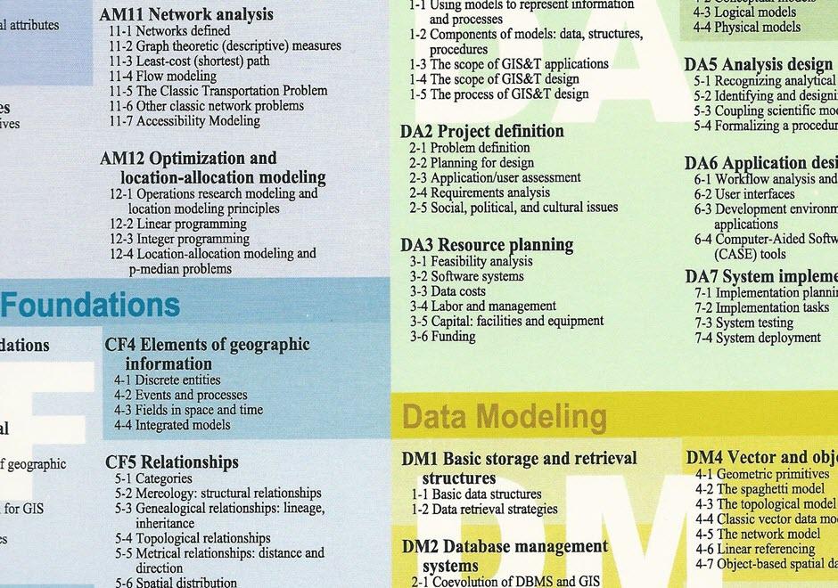
This knowledge area embodies a variety of data driven analytics, geocomputational methods, simulation and model driven approaches designed to study complex spatial-temporal problems, develop insights into characteristics of geospatial data sets, create and test geospatial process models, and construct knowledge of the behavior of geographically-explicit and dynamic processes and their patterns.

Topics in this Knowledge Area are listed thematically below. Existing topics are in regular font and linked directly to their original entries (published in 2006; these contain only Learning Objectives). Entries that have been updated and expanded are in bold. Forthcoming, future topics are italicized


Methodological Context Surface & Field Analyses Space-Time Analysis & Modeling
Geospatial Analysis & Model Building Modeling Surfaces Time Geography
Changing Context of GIScience Gridding, Interpolation, and Contouring Capturing Spatio-Temporal Dynamics in Computational Modeling 
Building Blocks Inverse Distance Weighting GIS-Based Computational Modeling
Overlay & Combination Operations Radial Basis & Spline Functions Computational Movement Analysis
Areal Interpolation Polynomial Functions Volumes and Space-Time Volumes
Aggregation of Spatial Entities Kriging Interpolation  
Classification & Clustering LiDAR Point Cloud Analysis Geocomputational Methods & Models
Boundaries & Zone Membership Intervisibility, Line-of-Sight, and Viewsheds Cellular Automata
Spatial Queries Digital Elevation Models & Terrain Metrics Agent-based Modeling
Buffers TIN-based Models and Terrain Metrics Simulation Modeling
Grid Operations & Map Algebra Watersheds & Drainage Networks Artificial Neural Networks
Data Exploration & Spatial Statistics 3D Parametric Surfaces Genetic Algorithms & Evolutionary Computing 
Spatial Statistics Network & Location Analysis Big Data & Geospatial Analysis
Spatial Sampling for Spatial Analysis Intro to Network & Location Analysis Problems of Large Spatial Databases
Exploratory Spatial Data Analysis (ESDA) Location & Service Area Problems Pattern Recognition & Matching
Point Pattern Analysis Network Route & Tour Problems Artificial Intelligence Approaches
Kernels & Density Estimation Modelling Accessibility Intro to Spatial Data Mining
Spatial Interaction Location-allocation Modeling Rule Learning for Spatial Data Mining
Cartographic Modeling The Classic Transportation Problem Machine Learning Approaches
Multi-criteria Evaluation   CyberGIS and Cyberinfrastructure
Grid-based Statistics and Metrics   Analysis of Errors & Uncertainty
Landscape Metrics   Error-based Uncertainty
Hot-spot and Cluster Analysis   Conceptual Models of Error & Uncertainty
Global Measures of Spatial Association   Spatial Data Uncertainty
Local Indicators of Spatial Autocorrelation   Problems of Scale & Zoning
Simple Regression & Trend Surface Analysis   Thematic Accuracy & Assessment
Geographically Weighted Regression   Stochastic Simulation & Monte Carlo Methods
Spatial Autoregressive Models   Mathematical Models of Uncertainty
Spatial Filtering Models   Fuzzy Aggregation Operators


AM-06 - Grid Operations and Map Algebra

Grid operations are manipulation and analytical computations performed on raster data. Map Algebra is a language for organizing and implementing grid operations in Geographic Information Systems (GIS) software, and is typically categorized into Local, Focal, and Zonal functions, where each function typically ingests one or more grids and outputs a new grid. The value of a specific grid cell in the output grid for Local functions is determined from the value(s) of the analogous cell position(s) in the input grid(s), for Focal functions from the grid cell values drawn from a neighborhood around the specific output grid cell, and for Zonal functions from a set of grid cells specified in a separate zone grid. Individual functions within a category vary by applying a different arithmetic, statistical, or other type of operator to the function. Map Algebra also includes Global and Block function categories. Grid operations can be categorized as data manipulation procedures or within domain-specific applications, such as terrain analysis or image processing. Grid operations are employed in a variety of GIS-based analyses, but are particularly widely used for suitability modeling and environmental analyses.

AM-17 - Intervisibility, Line-of-Sight, and Viewsheds
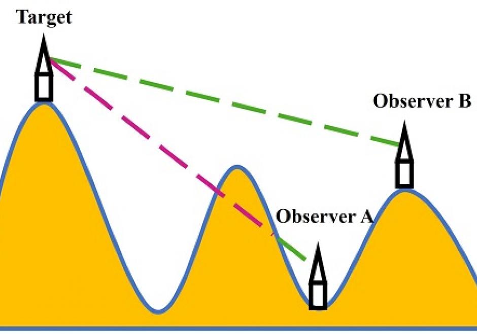
The visibility of a place refers to whether it can be seen by observers from one or multiple other locations. Modeling the visibility of points has various applications in GIS, such as placement of observation points, military observation, line-of-sight communication, optimal path route planning, and urban design. This chapter provides a brief introduction to visibility analysis, including an overview of basic conceptions in visibility analysis, the methods for computing intervisibility using discrete and continuous approaches based on DEM and TINs, the process of intervisibility analysis, viewshed and reverse viewshed analysis. Several practical applications involving visibility analysis are illustrated for geographical problem-solving. Finally, existing software and toolboxes for visibility analysis are introduced.

AM-08 - Kernels and Density Estimation

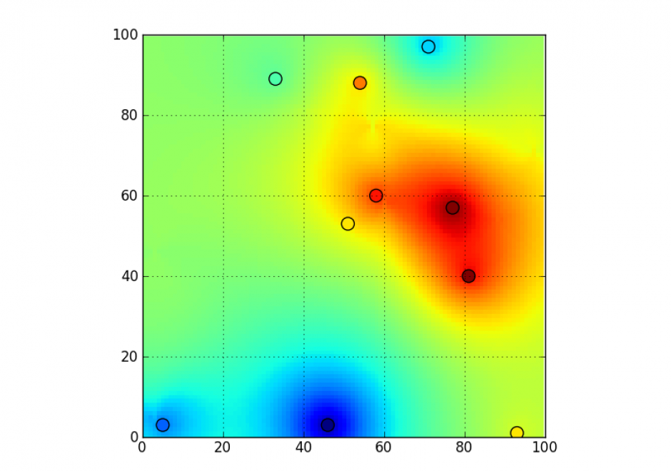
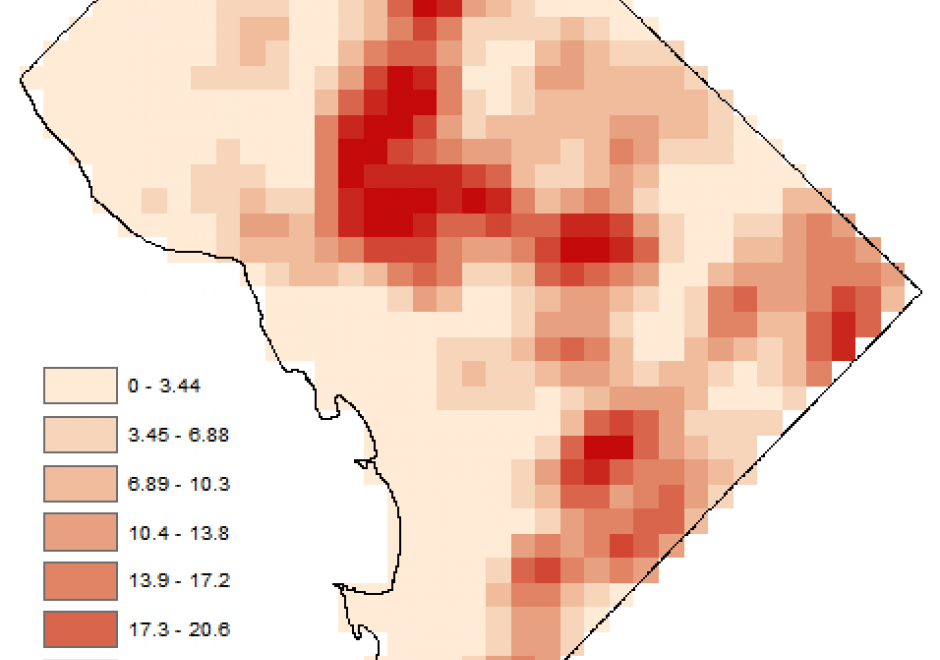
Kernel density estimation is an important nonparametric technique to estimate density from point-based or line-based data. It has been widely used for various purposes, such as point or line data smoothing, risk mapping, and hot spot detection. It applies a kernel function on each observation (point or line) and spreads the observation over the kernel window. The kernel density estimate at a location will be the sum of the fractions of all observations at that location. In a GIS environment, kernel density estimation usually results in a density surface where each cell is rendered based on the kernel density estimated at the cell center. The result of kernel density estimation could vary substantially depending on the choice of kernel function or kernel bandwidth, with the latter having a greater impact. When applying a fixed kernel bandwidth over all of the observations, undersmoothing of density may occur in areas with only sparse observation while oversmoothing may be found in other areas. To solve this issue, adaptive or variable bandwidth approaches have been suggested.

AM-29 - Kriging Interpolation

Kriging is an interpolation method that makes predictions at unsampled locations using a linear combination of observations at nearby sampled locations. The influence of each observation on the kriging prediction is based on several factors: 1) its geographical proximity to the unsampled location, 2) the spatial arrangement of all observations (i.e., data configuration, such as clustering of observations in oversampled areas), and 3) the pattern of spatial correlation of the data. The development of kriging models is meaningful only when data are spatially correlated.. Kriging has several advantages over traditional interpolation techniques, such as inverse distance weighting or nearest neighbor: 1) it provides a measure of uncertainty attached to the results (i.e., kriging variance); 2) it accounts for direction-dependent relationships (i.e., spatial anisotropy); 3) weights are assigned to observations based on the spatial correlation of data instead of assumptions made by the analyst for IDW; 4) kriging predictions are not constrained to the range of observations used for interpolation, and 5) data measured over different spatial supports can be combined and change of support, such as downscaling or upscaling, can be conducted.

AM-54 - Landscape Metrics

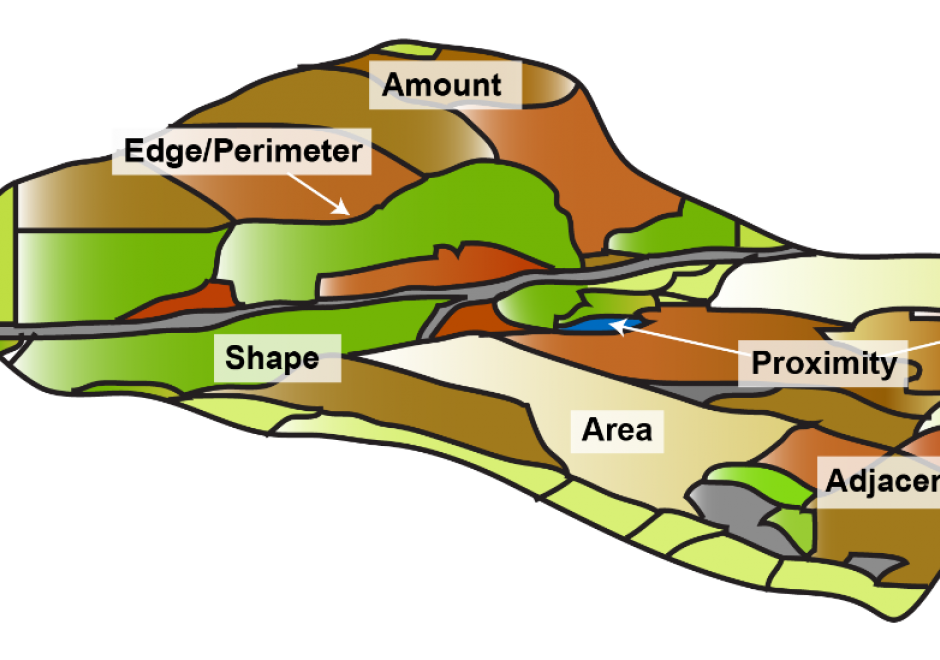
Landscape metrics are algorithms that quantify the spatial structure of patterns – primarily composition and configuration - within a geographic area. The term "landscape metrics" has historically referred to indices for categorical land cover maps, but with emerging datasets, tools, and software programs, the field is growing to include other types of landscape pattern analyses such as graph-based metrics, surface metrics, and three-dimensional metrics. The choice of which metrics to use requires careful consideration by the analyst, taking into account the data and application. Selecting the best metric for the problem at hand is not a trivial task given the large numbers of metrics that have been developed and software programs to implement them.

AM-23 - Local Measures of Spatial Association

Local measures of spatial association are statistics used to detect variations of a variable of interest across space when the spatial relationship of the variable is not constant across the study region, known as spatial non-stationarity or spatial heterogeneity. Unlike global measures that summarize the overall spatial autocorrelation of the study area in one single value, local measures of spatial association identify local clusters (observations nearby have similar attribute values) or spatial outliers (observations nearby have different attribute values). Like global measures, local indicators of spatial association (LISA), including local Moran’s I and local Geary’s C, incorporate both spatial proximity and attribute similarity. Getis-Ord Gi*another popular local statistic, identifies spatial clusters at various significance levels, known as hot spots (unusually high values) and cold spots (unusually low values). This so-called “hot spot analysis” has been extended to examine spatiotemporal trends in data. Bivariate local Moran’s I describes the statistical relationship between one variable at a location and a spatially lagged second variable at neighboring locations, and geographically weighted regression (GWR) allows regression coefficients to vary at each observation location. Visualization of local measures of spatial association is critical, allowing researchers of various disciplines to easily identify local pockets of interest for future examination.

AM-43 - Location and Service Area Problems

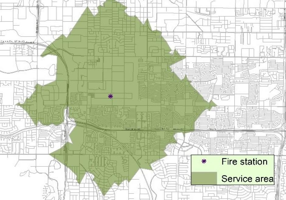
Many facilities exist to provide essential services in a city or region. The service area of a facility refers to a geographical area where the intended service of the facility can be received effectively. Service area delineation varies with the particular service a facility provides. This topic examines two types of service areas, one that can be defined based on a predetermined range such as travel distance/time and another based on the nearest facility available. Relevant location models are introduced to identify the best location(s) of one or multiple facilities to maximize service provision or minimize the system-wide cost. The delineation of service areas and structuring of a location model draw extensively on existing functions in a GIS. The topic represents an important area of GIS&T.

AM-46 - Location-allocation modeling

Location-allocation models involve two principal elements: 1) multiple facility location; and 2) the allocation of the services or products provided by those facilities to places of demand. Such models are used in the design of logistic systems like supply chains, especially warehouse and factory location, as well as in the location of public services. Public service location models involve objectives that often maximize access and levels of service, while private sector applications usually attempt to minimize cost. Such models are often hard to solve and involve the use of integer-linear programming software or sophisticated heuristics. Some models can be solved with functionality provided in GIS packages and other models are applied, loosely coupled, with GIS. We provide a short description of formulating two different models as well as discuss how they are solved.

AM-94 - Machine Learning Approaches

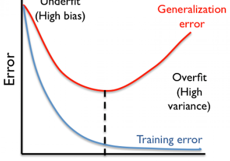
Machine learning approaches are increasingly used across numerous applications in order to learn from data and generate new knowledge discoveries, advance scientific studies and support automated decision making. In this knowledge entry, the fundamentals of Machine Learning (ML) are introduced, focusing on how feature spaces, models and algorithms are being developed and applied in geospatial studies. An example of a ML workflow for supervised/unsupervised learning is also introduced. The main challenges in ML approaches and our vision for future work are discussed at the end.

AM-48 - Mathematical models of uncertainty: probability and statistics
  • Devise simple ways to represent probability information in GIS
  • Describe the basic principles of randomness and probability
  • Compute descriptive statistics and geostatistics of geographic data
  • Interpret descriptive statistics and geostatistics of geographic data
  • Recognize the assumptions underlying probability and geostatistics and the situations in which they are useful analytical tools

Pages