2021 QUARTER 03

A B C D E F G H I J K L M N O P R S T U V W
DM-23 - Fields in space and time
  • Define a field in terms of properties, space, and time
  • Formalize the notion of field using mathematical functions and calculus
  • Recognize the influences of scale on the perception and meaning of fields
  • Evaluate the field view’s description of “objects” as conceptual discretizations of continuous patterns
  • Identify applications and phenomena that are not adequately modeled by the field view
  • Identify examples of discrete and continuous change found in spatial, temporal, and spatio-temporal fields
  • Relate the notion of field in GIS to the mathematical notions of scalar and vector fields
  • Differentiate various sources of fields, such as substance properties (e.g., temperature), artificial constructs (e.g., population density), and fields of potential or influence (e.g., gravity)
CV-31 - Flow Maps

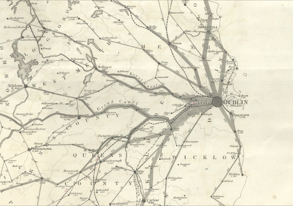
Flow mapping is a cartographic method of representing movement of phenomena. Maps of this type often depict the vector movement of entities (imports and exports, people, information) between geographic areas, but the general method also encompasses a range of graphics illustrating networks (e.g., transit and communications grids) and dynamic systems (e.g., wind and water currents). Most flow maps typically use line symbols of varying widths, lengths, shapes, colors, or speeds (in the case of animated flow maps) to show the quality, direction, and magnitude of movements. Aesthetic considerations for flow maps are numerous and their production is often done manually without significant automation. Flow maps frequently use distorted underlying geography to accommodate the placement of flow paths, which are often dramatically smoothed/abstracted into visually pleasing curves or simply straight lines. In the extreme, such maps lack a geographic coordinate space and are more diagrammatic, as in Sankey diagrams, alluvial diagrams, slope graphs, and circle migration plots. Whatever their form, good flow maps should effectively visualize the relative magnitude and direction of movement or potential movement between a one or more origins and destinations.

KE-11 - Funding
  • Identify potential sources of funding (internal and external) for a project or enterprise GIS
  • Create proposals and presentations to secure funding
  • Analyze previous attempts at funding to identify successful and unsuccessful techniques
AM-88 - Fuzzy aggregation operators
  • Compare and contrast Boolean and fuzzy logical operations
  • Compare and contrast several operators for fuzzy aggregation, including those for intersect and union
  • Exemplify one use of fuzzy aggregation operators
  • Describe how an approach to map overlay analysis might be different if region boundaries were fuzzy rather than crisp
  • Describe fuzzy aggregation operators
DM-41 - Fuzzy logic
  • Describe how linear functions are used to fuzzify input data (i.e., mapping domain values to linguistic variables)
  • Support or refute the statement by Lotfi Zadeh, that “As complexity rises, precise statements lose meaning and meaningful statements lose precision,” as it relates to GIS&T
  • Explain why fuzzy logic, rather then Boolean algebra models, can be useful for representing real world boundaries between different tree species
PD-33 - GDAL/OGR and Geospatial Data IO Libraries

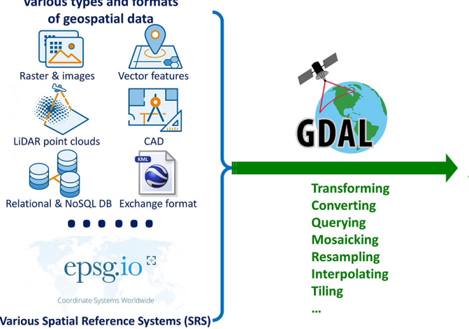
Manipulating (e.g., reading, writing, and processing) geospatial data, the first step in geospatial analysis tasks, is a complicated step, especially given the diverse types and formats of geospatial data combined with diverse spatial reference systems. Geospatial data Input/Output (IO) libraries help facilitate this step by handling some technical details of the IO process. GDAL/OGR is the most widely-used, broadly-supported, and constantly-updated free library among existing geospatial data IO libraries. GDAL/OGR provides a single raster abstract data model and a single vector abstract data model for processing and analyzing raster and vector geospatial data, respectively, and it supports most, if not all, commonly-used geospatial data formats. GDAL/OGR can also perform both cartographic projections on large scales and coordinate transformation for most of the spatial reference systems used in practice. This entry provides an overview of GDAL/OGR, including why we need such a geospatial data IO library and how it can be applied to various formats of geospatial data to support geospatial analysis tasks. Alternative geospatial data IO libraries are also introduced briefly. Future directions of development for GDAL/OGR and other geospatial data IO libraries in the age of big data and cloud computing are discussed as an epilogue to this entry.

DM-27 - Genealogical relationships: lineage, inheritance
  • Describe ways in which a geographic entity can be created from one or more others
  • Discuss the effects of temporal scale on the modeling of genealogical structures
  • Describe the genealogy (as identity-based change or temporal relationships) of particular geographic phenomena
  • Determine whether it is important to represent the genealogy of entities for a particular application
AM-78 - Genetic Algorithms and Evolutionary Computing

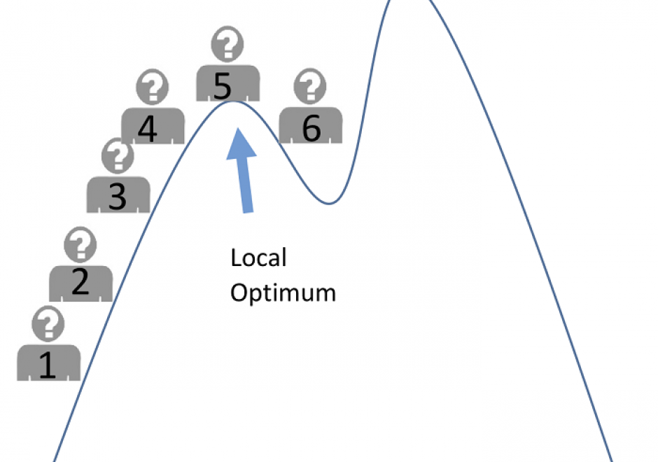
Genetic algorithms (GAs) are a family of search methods that have been shown to be effective in finding optimal or near-optimal solutions to a wide range of optimization problems. A GA maintains a population of solutions to the problem being solved and uses crossover, mutation, and selection operations to iteratively modify them. As the population evolves across generations, better solutions are created and inferior ones are selectively discarded. GAs usually run for a fixed number of iterations (generations) or until further improvements do not obtain. This contribution discusses the fundamental principles of genetic algorithms and uses Python code to illustrate how GAs can be developed for both numerical and spatial optimization problems. Computational experiments are used to demonstrate the effectiveness of GAs and to illustrate some nuances in GA design.

DM-47 - Geographic coordinate system
  • Distinguish between various latitude definitions (e.g., geocentric, geodetic, astronomic latitudes)
  • Explain the angular measurements represented by latitude and longitude coordinates
  • Calculate the latitude and longitude coordinates of a given location on the map using the coordinate grid ticks in the collar of a topographic map and the appropriate interpolation formula
  • Mathematically express the relationship between Cartesian coordinates and polar coordinates
  • Calculate the uncertainty of a ground position defined by latitude and longitude coordinates specified in decimal degrees to a given number of decimal places
  • Use GIS software and base data encoded as geographic coordinates to geocode a list of address-referenced locations
  • Locate on a globe the positions represented by latitude and longitude coordinates
  • Write an algorithm that converts geographic coordinates from decimal degrees (DD) to degrees, minutes, seconds (DMS) format
FC-22 - Geometric Primitives and Algorithms

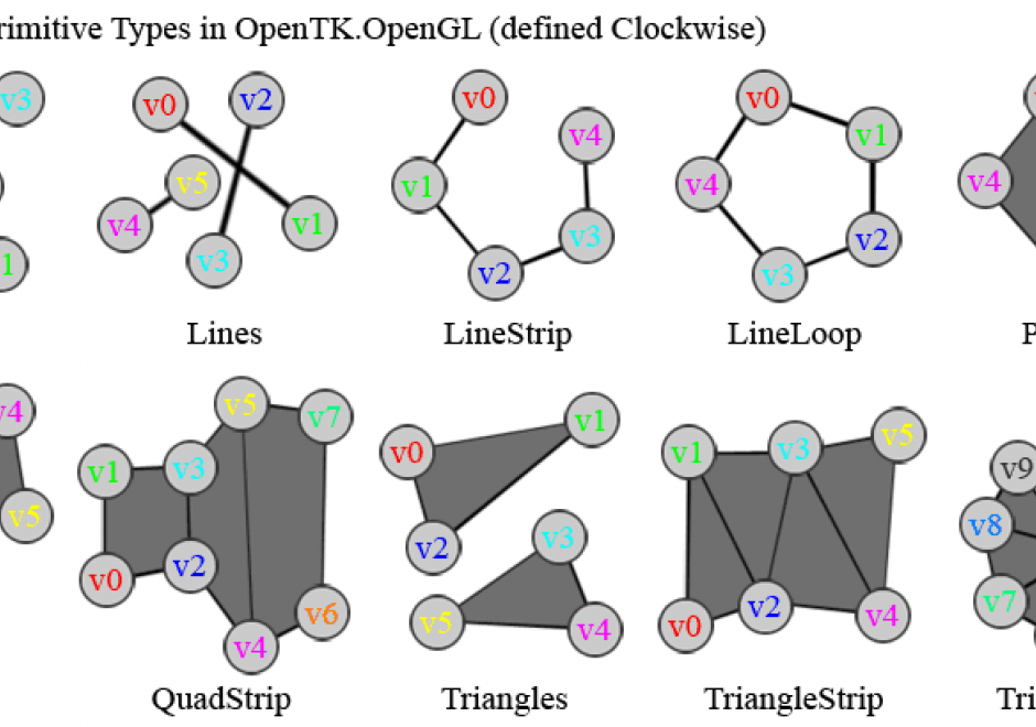
Geometric primitives are the representations used and computations performed in a GIS that concern the spatial aspects of the data, data objects described by coordinates. In vector geometry, we distinguish in zero-, one-, two-, and three-dimensional objects, better known as points, linear features, areal or planar features, and volumetric features. A GIS stores and performs computations on all of these. Often, planar features form a collective known as a (spatial) subdivision. Computations on geometric objects show up in data simplification, neighborhood analysis, spatial clustering, spatial interpolation, automated text placement, segmentation of trajectories, map matching, and many other tasks. They should be contrasted with computations on attributes or networks.

There are various kinds of vector data models for subdivisions. The classical ones are known as spaghetti and pizza models, but nowadays it is recognized that topological data models are the representation of choice. We overview these models briefly.

Computations range from simple to highly complex: deciding whether a point lies in a rectangle needs four comparisons, whereas performing map overlay on two subdivisions requires advanced knowledge of algorithm design. We introduce map overlay, Voronoi diagrams, and Delaunay triangulations and mention algorithmic approaches to compute them.

Pages