spatial statistics

FC-37 - Spatial Autocorrelation

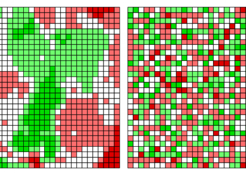
The scientific term spatial autocorrelation describes Tobler’s first law of geography: everything is related to everything else, but nearby things are more related than distant things. Spatial autocorrelation has a:

  • past characterized by scientists’ non-verbal awareness of it, followed by its formalization;
  • present typified by its dissemination across numerous disciplines, its explication, its visualization, and its extension to non-normal data; and
  • an anticipated future in which it becomes a standard in data analytic computer software packages, as well as a routinely considered feature of space-time data and in spatial optimization practice.

Positive spatial autocorrelation constitutes the focal point of its past and present; one expectation is that negative spatial autocorrelation will become a focal point of its future.

AM-25 - Bayesian methods
  • Define “prior and posterior distributions” and “Markov-Chain Monte Carlo”
  • Explain how the Bayesian perspective is a unified framework from which to view uncertainty
  • Compare and contrast Bayesian methods and classical “frequentist” statistical methods
AM-23 - Local measures of spatial association
  • Describe the effect of non-stationarity on local indices of spatial association
  • Decompose Moran’s I and Geary’s c into local measures of spatial association
  • Compute the Gi and Gi* statistics
  • Explain how geographically weighted regression provides a local measure of spatial association
  • Explain how a weights matrix can be used to convert any classical statistic into a local measure of spatial association
  • Compare and contrast global and local statistics and their uses
AM-22 - Global measures of spatial association
  • Describe the effect of the assumption of stationarity on global measures of spatial association
  • Justify, compute, and test the significance of the join count statistic for a pattern of objects
  • Compute the K function
  • Explain how a statistic that is based on combining all the spatial data and returning a single summary value or two can be useful in understanding broad spatial trends
  • Compute measures of overall dispersion and clustering of point datasets using nearest neighbor distance statistics
  • Compute Moran’s I and Geary’s c for patterns of attribute data measured on interval/ratio scales
  • Explain how the K function provides a scale-dependent measure of dispersion
AM-19 - Exploratory data analysis (EDA)
  • Describe the statistical characteristics of a set of spatial data using a variety of graphs and plots (including scatterplots, histograms, boxplots, q–q plots)
  • Select the appropriate statistical methods for the analysis of given spatial datasets by first exploring them using graphic methods
FC-37 - Spatial Autocorrelation

The scientific term spatial autocorrelation describes Tobler’s first law of geography: everything is related to everything else, but nearby things are more related than distant things. Spatial autocorrelation has a:

  • past characterized by scientists’ non-verbal awareness of it, followed by its formalization;
  • present typified by its dissemination across numerous disciplines, its explication, its visualization, and its extension to non-normal data; and
  • an anticipated future in which it becomes a standard in data analytic computer software packages, as well as a routinely considered feature of space-time data and in spatial optimization practice.

Positive spatial autocorrelation constitutes the focal point of its past and present; one expectation is that negative spatial autocorrelation will become a focal point of its future.

AM-22 - Global measures of spatial association
  • Describe the effect of the assumption of stationarity on global measures of spatial association
  • Justify, compute, and test the significance of the join count statistic for a pattern of objects
  • Compute the K function
  • Explain how a statistic that is based on combining all the spatial data and returning a single summary value or two can be useful in understanding broad spatial trends
  • Compute measures of overall dispersion and clustering of point datasets using nearest neighbor distance statistics
  • Compute Moran’s I and Geary’s c for patterns of attribute data measured on interval/ratio scales
  • Explain how the K function provides a scale-dependent measure of dispersion
AM-25 - Bayesian methods
  • Define “prior and posterior distributions” and “Markov-Chain Monte Carlo”
  • Explain how the Bayesian perspective is a unified framework from which to view uncertainty
  • Compare and contrast Bayesian methods and classical “frequentist” statistical methods
AM-24 - Outliers
  • Explain how outliers affect the results of analyses
  • Explain how the following techniques can be used to examine outliers: tabulation, histograms, box plots, correlation analysis, scatter plots, local statistics
AM-23 - Local measures of spatial association
  • Describe the effect of non-stationarity on local indices of spatial association
  • Decompose Moran’s I and Geary’s c into local measures of spatial association
  • Compute the Gi and Gi* statistics
  • Explain how geographically weighted regression provides a local measure of spatial association
  • Explain how a weights matrix can be used to convert any classical statistic into a local measure of spatial association
  • Compare and contrast global and local statistics and their uses

Pages