2019 QUARTER 04

A B C D E F G H I K L M N O P R S T U V W
AM-16 - Interpolation methods
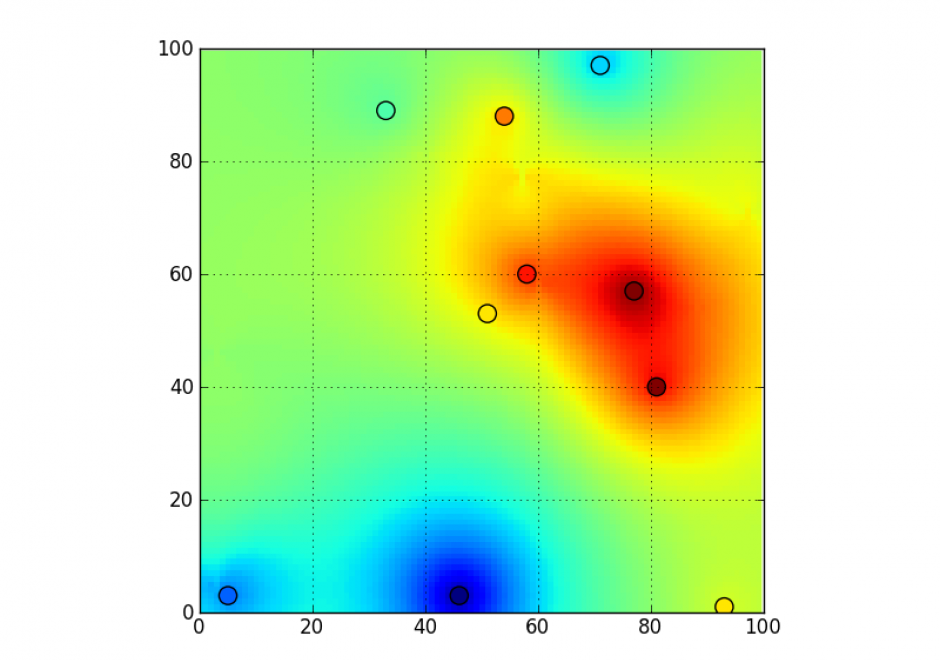
  • Identify the spatial concepts that are assumed in different interpolation algorithms
  • Compare and contrast interpolation by inverse distance weighting, bi-cubic spline fitting, and kriging
  • Differentiate between trend surface analysis and deterministic spatial interpolation
  • Explain why different interpolation algorithms produce different results and suggest ways by which these can be evaluated in the context of a specific problem
  • Design an algorithm that interpolates irregular point elevation data onto a regular grid
  • Outline algorithms to produce repeatable contour-type lines from point datasets using proximity polygons, spatial averages, or inverse distance weighting
  • Implement a trend surface analysis using either the supplied function in a GIS or a regression function from any standard statistical package
  • Describe how surfaces can be interpolated using splines
  • Explain how the elevation values in a digital elevation model (DEM) are derived by interpolation from irregular arrays of spot elevations
  • Discuss the pitfalls of using secondary data that has been generated using interpolations (e.g., Level 1 USGS DEMs)
  • Estimate a value between two known values using linear interpolation (e.g., spot elevations, population between census years)
AM-17 - Intervisibility
  • Define “intervisibility”
  • Outline an algorithm to determine the viewshed (area visible) from specific locations on surfaces specified by DEMs
  • Perform siting analyses using specified visibility, slope, and other surface related constraints
  • Explain the sources and impact of errors that affect intervisibility analyses
AM-08 - Kernels and density estimation
  • Describe the relationships between kernels and classical spatial interaction approaches, such as surfaces of potential
  • Outline the likely effects on analysis results of variations in the kernel function used and the bandwidth adopted
  • Explain why and how density estimation transforms point data into a field representation
  • Explain why, in some cases, an adaptive bandwidth might be employed
  • Create density maps from point datasets using kernels and density estimation techniques using standard software
  • Differentiate between kernel density estimation and spatial interpolation
AM-37 - Knowledge discovery
  • Explain how spatial data mining techniques can be used for knowledge discovery
  • Explain how a Bayesian framework can incorporate expert knowledge in order to retrieve all relevant datasets given an initial user query
  • Explain how visual data exploration can be combined with data mining techniques as a means of discovering research hypotheses in large spatial datasets
AM-29 - Kriging Interpolation

Kriging is an interpolation method that makes predictions at unsampled locations using a linear combination of observations at nearby sampled locations. The influence of each observation on the kriging prediction is based on several factors: 1) its geographical proximity to the unsampled location, 2) the spatial arrangement of all observations (i.e., data configuration, such as clustering of observations in oversampled areas), and 3) the pattern of spatial correlation of the data. The development of kriging models is meaningful only when data are spatially correlated.. Kriging has several advantages over traditional interpolation techniques, such as inverse distance weighting or nearest neighbor: 1) it provides a measure of uncertainty attached to the results (i.e., kriging variance); 2) it accounts for direction-dependent relationships (i.e., spatial anisotropy); 3) weights are assigned to observations based on the spatial correlation of data instead of assumptions made by the analyst for IDW; 4) kriging predictions are not constrained to the range of observations used for interpolation, and 5) data measured over different spatial supports can be combined and change of support, such as downscaling or upscaling, can be conducted.

DC-02 - Land records
  • Distinguish between GIS, LIS, and CAD/CAM in the context of land records management
  • Evaluate the difference in accuracy requirements for deeds systems versus registration systems
  • Exemplify and compare deed descriptions in terms of how accurately they convey the geometry of a parcel
  • Distinguish between topological fidelity and geometric accuracy in the context of a plat map
AM-54 - Landscape Metrics

Landscape metrics are algorithms that quantify the spatial structure of patterns – primarily composition and configuration - within a geographic area. The term "landscape metrics" has historically referred to indices for categorical land cover maps, but with emerging datasets, tools, and software programs, the field is growing to include other types of landscape pattern analyses such as graph-based metrics, surface metrics, and three-dimensional metrics. The choice of which metrics to use requires careful consideration by the analyst, taking into account the data and application. Selecting the best metric for the problem at hand is not a trivial task given the large numbers of metrics that have been developed and software programs to implement them.

Pages