All Topics

A B C D E F G H I J K L M N O P R S T U V W
DC-32 - Landsat

The Landsat series of satellites have collected the longest and continuous earth observation data. Earth surface data collected since 1972 are providing invaluable data for managing natural resources, monitoring changes, and disaster response. After the US Geological Survey (USGS) opened the entire archive to users, the number of monitoring and mapping applications have increased several folds. Currently, Landsat data can be obtained from the USGS and other private entities. The sensors onboard these Landsat satellites have improved over time resulting in changes to the spatial, spectral, radiometric, and temporal resolutions of the images they have collected. Data recorded by the sensors in the form of pixels can be converted to reflectance values. Recently, USGS has reprocessed the entire Landsat data archive and is releasing them as collections. This section provides an overview of the Landsat program and remotely sensed data characteristics, followed by the description of various sensors onboard and data collected by the past and current sensors.

AM-54 - Landscape Metrics
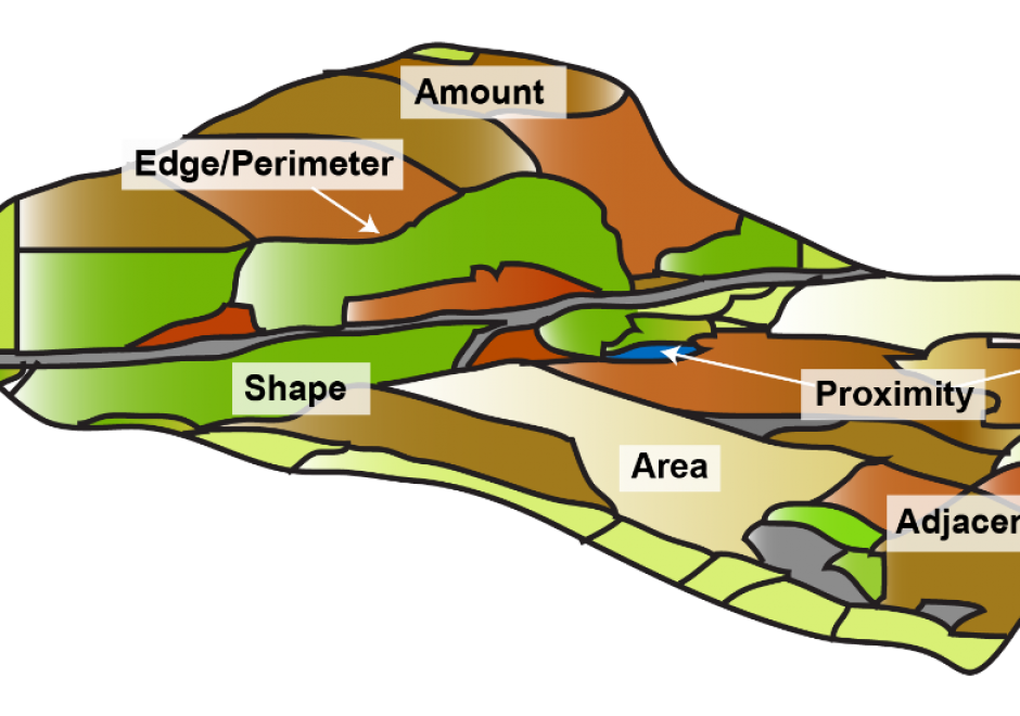
Landscape metrics are algorithms that quantify the spatial structure of patterns – primarily composition and configuration - within a geographic area. The term "landscape metrics" has historically referred to indices for categorical land cover maps, but with emerging datasets, tools, and software programs, the field is growing to include other types of landscape pattern analyses such as graph-based metrics, surface metrics, and three-dimensional metrics. The choice of which metrics to use requires careful consideration by the analyst, taking into account the data and application. Selecting the best metric for the problem at hand is not a trivial task given the large numbers of metrics that have been developed and software programs to implement them.

CV-28 - Lesson Design in Cartography Education

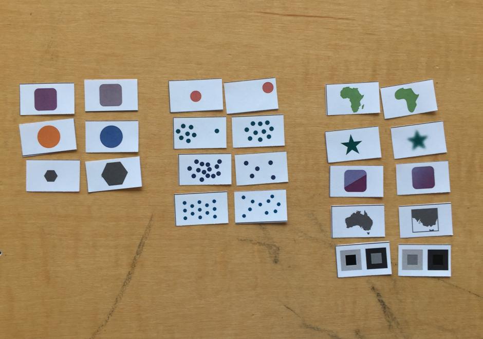
This entry describes six general variables of lesson design in cartography education and offers some practical advice for the development of materials for teaching cartography. First, a lesson’s scope concerns the set of ideas included in a lesson and helps identify different types of lessons based on the kinds of knowledge that they contain. Second, learning objectives concern the things that students should be able to do following a lesson and relate to different cognitive processes of learning. Third, a lesson’s scheme deals with the organizational framework for delivering content. Fourth, a lesson’s guidance concerns the amount and quality of supportive information provided. Fifth, a lesson’s sequence may involve one or more strategies for ordering content. Sixth, a lesson’s activity concerns what students do during a lesson and is often associated with different learning outcomes. These six variables help differentiate traditions for teaching cartography, elucidate some of the recurring challenges in cartography education, and offer strategies for designing lessons to foster meaningful learning outcomes.

DC-27 - Light Detection and Ranging (LiDAR)

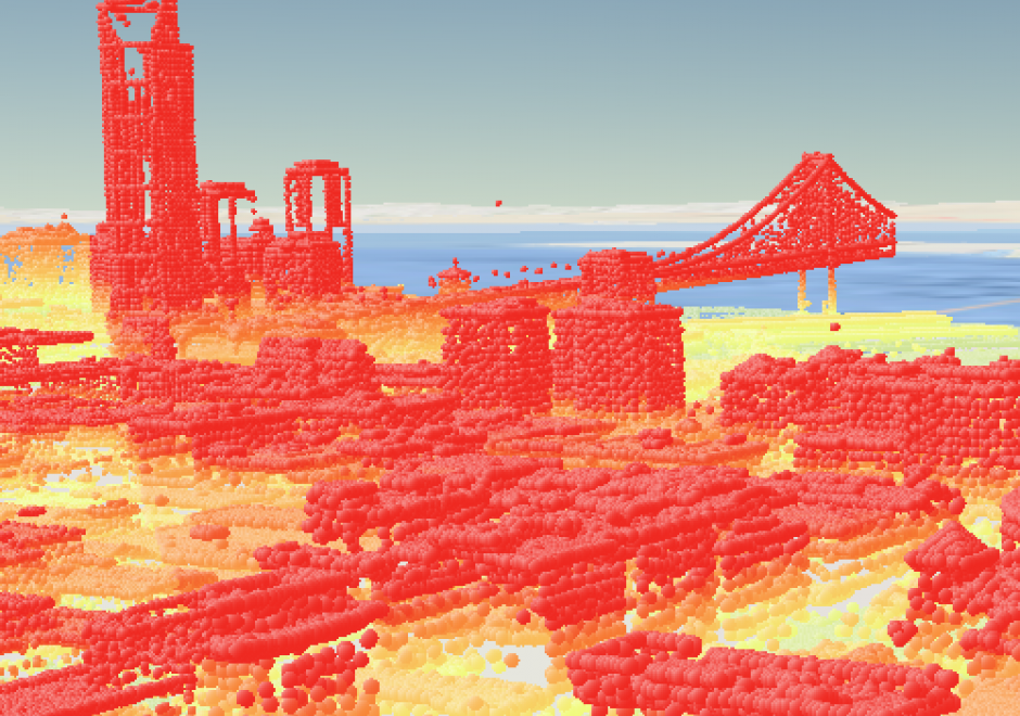
LiDAR (Light Detection and Ranging) is a remote sensing technology that collects information reflected or refracted from the Earth’s surface. The instrumentation that collects LiDAR data can be housed on drones, airplanes, helicopters, or satellites, and consists of a laser scanner that transmits pulses of light. These transmitted pulses reflect or refract from objects on the Earth’s surface or from the surface itself, and the time delay is recorded. Knowing the travel time and the speed of light, an elevation of each pulse above the surface can be determined. From the pulse data collected, the user can determine the topography and landscape features of the Earth or whatever surface has received the pulses. The evolution of software that displays and analyzes LiDAR data and the development of new and more compact file formats have allowed the use of LiDAR to grow dramatically in recent years.

PD-01 - Linear Programming and GIS

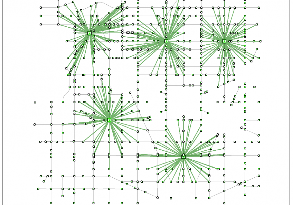
Linear programming is a set of methods for finding optimal solutions to mathematical models composed of a set of linear functions. Many spatial location problems can be structured as linear programs. However, even modest-sized problem instances can be very difficult to solve due to the combinatorial complexity of the problems and the associated computational expense that they incur. Geographic Information Systems software does not typically incorporate formal linear programming functionality, and instead commonly uses heuristic solution procedures to generate near-optimal solutions quickly. There is growing interest in integrating the spatial analytic tools incorporated in Geographic Information Systems with the solution power of linear programming software to generate guaranteed optimal solutions to spatial location problems.

DM-16 - Linear Referencing

Linear referencing is a term that encompasses a family of concepts and techniques for associating features with a spatial location along a network, rather than referencing those locations to a traditional spherical or planar coordinate system. Linear referencing is used when the location on the network, and the relationships to other locations on the network, are more significant than the location in 2D or 3D space. Linear referencing is commonly used in transportation applications, including roads, railways, and pipelines, although any network structure can be used as the basis for linearly referenced features. Several data models for storing linearly referenced data are available, and well-defined sets of procedures can be used to implement linear referencing for a particular application. As network analysis and network based statistical analysis become more prevalent across disciplines, linear referencing is likely to remain an important component of the data used for such analyses.

AM-23 - Local Measures of Spatial Association

Local measures of spatial association are statistics used to detect variations of a variable of interest across space when the spatial relationship of the variable is not constant across the study region, known as spatial non-stationarity or spatial heterogeneity. Unlike global measures that summarize the overall spatial autocorrelation of the study area in one single value, local measures of spatial association identify local clusters (observations nearby have similar attribute values) or spatial outliers (observations nearby have different attribute values). Like global measures, local indicators of spatial association (LISA), including local Moran’s I and local Geary’s C, incorporate both spatial proximity and attribute similarity. Getis-Ord Gi*another popular local statistic, identifies spatial clusters at various significance levels, known as hot spots (unusually high values) and cold spots (unusually low values). This so-called “hot spot analysis” has been extended to examine spatiotemporal trends in data. Bivariate local Moran’s I describes the statistical relationship between one variable at a location and a spatially lagged second variable at neighboring locations, and geographically weighted regression (GWR) allows regression coefficients to vary at each observation location. Visualization of local measures of spatial association is critical, allowing researchers of various disciplines to easily identify local pockets of interest for future examination.

AM-43 - Location and Service Area Problems

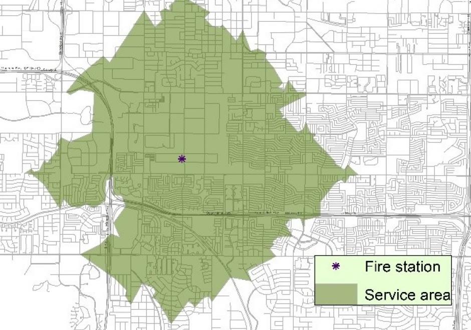
Many facilities exist to provide essential services in a city or region. The service area of a facility refers to a geographical area where the intended service of the facility can be received effectively. Service area delineation varies with the particular service a facility provides. This topic examines two types of service areas, one that can be defined based on a predetermined range such as travel distance/time and another based on the nearest facility available. Relevant location models are introduced to identify the best location(s) of one or multiple facilities to maximize service provision or minimize the system-wide cost. The delineation of service areas and structuring of a location model draw extensively on existing functions in a GIS. The topic represents an important area of GIS&T.

GS-04 - Location Privacy

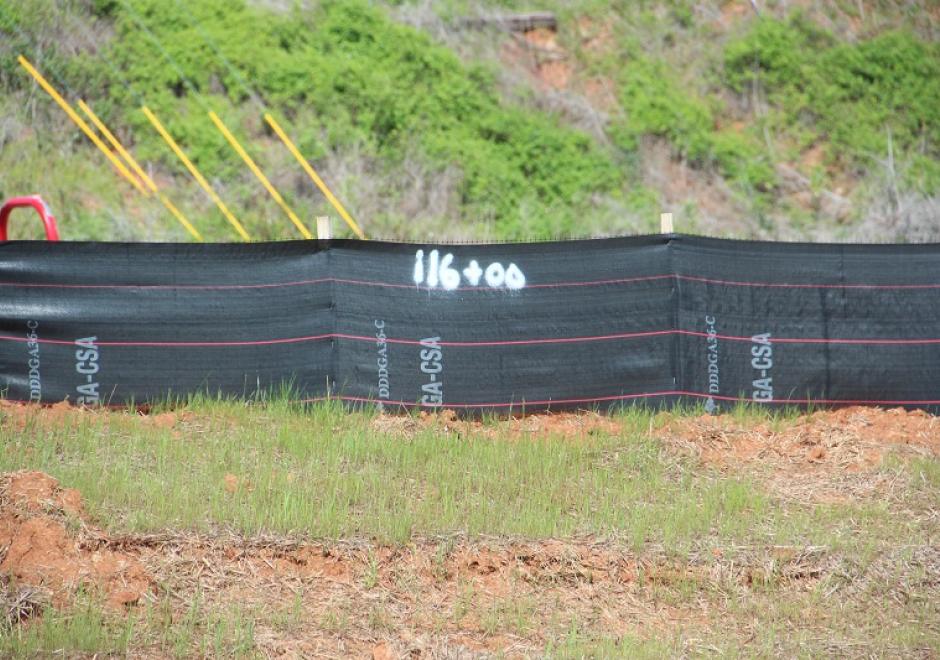
How effective is this fence at keeping people, objects, or sensitive information inside or outside? Location Privacy is concerned with the claim of individuals to determine when, how, and to what extent information about themselves and their location is communicated to others. Privacy implications for spatial data are growing in importance with growing awareness of the value of geo-information and the advent of the Internet of Things, Cloud-Based GIS, and Location Based Services.  

In the rapidly changing landscape of GIS and public domain spatial data, issues of location privacy are more important now than ever before. Technological trailblazing tends to precede legal safeguards. The development of GIS tools and the work of the GIS&T research and user community have typically occurred at a much faster rate than the establishment of legislative frameworks governing the use of spatial data, including privacy concerns. Yet even in a collaborative environment that characterizes the GIS&T community, and despite progress made, the issue of location privacy is a particularly thorny one, occurring as it does at the intersection of geotechnology and society.

AM-46 - Location-allocation modeling

Location-allocation models involve two principal elements: 1) multiple facility location; and 2) the allocation of the services or products provided by those facilities to places of demand. Such models are used in the design of logistic systems like supply chains, especially warehouse and factory location, as well as in the location of public services. Public service location models involve objectives that often maximize access and levels of service, while private sector applications usually attempt to minimize cost. Such models are often hard to solve and involve the use of integer-linear programming software or sophisticated heuristics. Some models can be solved with functionality provided in GIS packages and other models are applied, loosely coupled, with GIS. We provide a short description of formulating two different models as well as discuss how they are solved.

Pages